Vectorial diffraction: longitudinal fields, vector beams and high NA foci

The scalar propagators treat each Cartesian field component on its own. That is fine as long as all plane waves of a beam travel almost along \(z\). For strongly diverging beams (small waists, high numerical apertures) it misses something: an electromagnetic wave is transverse, \(\mathbf{k}\cdot\mathbf{E} = 0\) for every plane wave, so tilted plane waves carry a longitudinal component \(E_z\). This notebook shows the vectorial tools of pyoptics.propagators:

Function	What it does
longitudinal_component(E_x, E_y, x, y, wl, n)	\(E_z\) from the transverse components via \(\nabla\cdot\mathbf{E} = 0\): \(\tilde E_z = -(k_x\tilde E_x + k_y\tilde E_y)/k_z\)
vectorial_rayleigh_sommerfeld_TF(field, x, y, z, wl, n)	exact angular spectrum propagation of a field \([E_x, E_y]\) given in a plane; returns \([E_x, E_y, E_z]\)
propagate_vectorial(propagator, field, ...)	any scalar propagator for \(E_x, E_y\), plus \(E_z\) (from \(\nabla\cdot\mathbf{E}=0\), or \(\mathbf{E}\cdot\mathbf{r} = 0\) for fraunhofer())
propagate_padded(...)	also accepts vector fields of shape (Ny, Nx, 2) or (Ny, Nx, 3)
vectorial_mansuripur(field, x, y, z, wl, n)	Mansuripur’s method for the focus of an aplanatic high NA lens (Richards-Wolf theory)
aplanatic_rotation(sigma_x, sigma_y)	the polarization rotation of a ray bent by an aplanatic lens

Vector fields are arrays of shape (Ny, Nx, 2) with \([E_x, E_y]\) or (Ny, Nx, 3) with \([E_x, E_y, E_z]\). Convention as everywhere in pyoptics: fields vary as \(\exp(i(\mathbf{k}\cdot\mathbf{r} - \omega t))\). All lengths are in units of the wavelength.

import functools

import numpy as np
import matplotlib.pyplot as plt
from scipy.integrate import quad
from scipy.special import jv, j1

from pyoptics.fft import FT, inv_FT
from pyoptics.propagators import (longitudinal_component, vectorial_rayleigh_sommerfeld_TF,
                                  propagate_vectorial, propagate_padded, vectorial_mansuripur,
                                  aplanatic_rotation, rayleigh_sommerfeld_I_TF, fresnel_TF,
                                  fraunhofer)
from pyoptics.utils import grid1d, freq_grid

plt.rcParams.update({"figure.dpi": 100, "image.origin": "lower", "font.size": 11})

wl = 1.0
k = 2*np.pi/wl

def grid(L, N):
    x = grid1d(-L/2, L/2, N)
    return x, x, *np.meshgrid(x, x)

def components(E):
    return [np.abs(E[:, :, i])**2 for i in range(3)]

def show_components(E, x, y, title, extent_half=None, fig_title=None, total=True):
    """Plot |E_x|², |E_y|², |E_z|² (and the sum) normalized to the peak of the sum."""
    I = components(E)
    I_tot = sum(I)
    m = I_tot.max()
    panels = I + ([I_tot] if total else [])
    names = ["$|E_x|^2$", "$|E_y|^2$", "$|E_z|^2$", "$|\\mathbf{E}|^2$"]
    fig, axes = plt.subplots(1, len(panels), figsize=(3.6*len(panels), 3.4))
    ext = [x[0], x[-1], y[0], y[-1]]
    for ax, img, name in zip(axes, panels, names):
        vmax = img.max()/m if img.max()/m > 1e-6 else 1.0   # identically zero: plain black panel
        im = ax.imshow(img/m, extent=ext, cmap="inferno", vmin=0, vmax=vmax)
        ax.set_title(f"{name}  (peak {img.max()/m:.3f})", fontsize=10)
        ax.set_xlabel("x [λ]")
        if extent_half:
            ax.set_xlim(-extent_half, extent_half); ax.set_ylim(-extent_half, extent_half)
        fig.colorbar(im, ax=ax, shrink=0.8)
    axes[0].set_ylabel("y [λ]")
    fig.suptitle(fig_title or title)
    fig.tight_layout()
    return fig

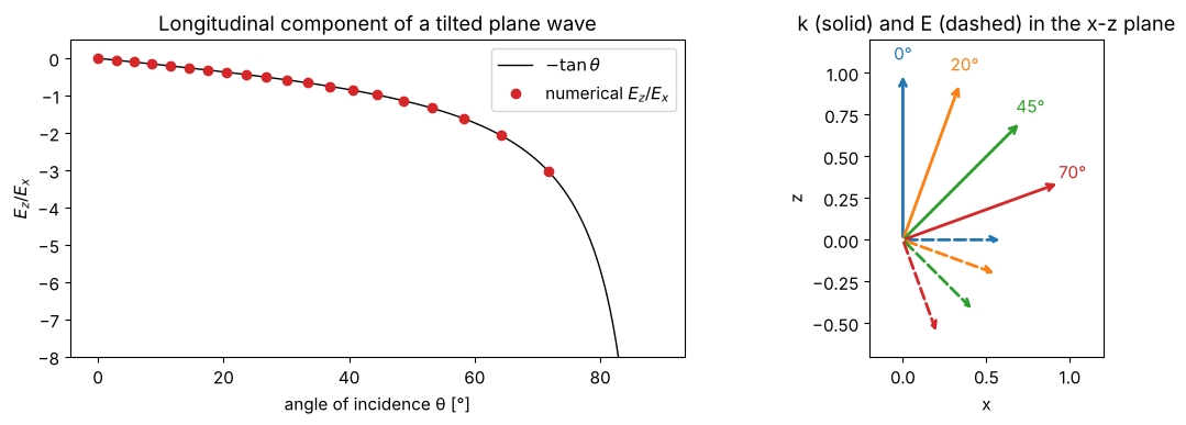
1. The longitudinal field of a tilted plane wave

A plane wave \(\exp(i(k_x x + k_z z))\) that is polarized in the \(x\)-\(z\) plane has \(E_z = -E_x k_x/k_z = -E_x\tan\theta\). longitudinal_component() finds this from \(E_x\) alone. The plane waves are chosen on the frequency grid of the window, so the FFT represents them exactly.

x, y, X, Y = grid(20.0, 128)
m_vals = np.arange(0, 20)
kx_vals = 2*np.pi*m_vals/20.0
theta = np.arcsin(kx_vals/k)
ratio = []
for kx in kx_vals:
    E_x = np.exp(1j*kx*X)
    E_z = longitudinal_component(E_x, 0*E_x, x, y, wl)
    ratio.append((E_z/E_x)[64, 64])
ratio = np.array(ratio)

fig, axes = plt.subplots(1, 2, figsize=(12, 4))
th = np.linspace(0, 89, 400)
axes[0].plot(th, -np.tan(np.radians(th)), "k-", lw=1, label="$-\\tan\\theta$")
axes[0].plot(np.degrees(theta), ratio.real, "o", color="C3", label="numerical $E_z/E_x$")
axes[0].set_ylim(-8, 0.5); axes[0].set_xlabel("angle of incidence θ [°]"); axes[0].set_ylabel("$E_z/E_x$")
axes[0].legend(); axes[0].set_title("Longitudinal component of a tilted plane wave")

# the field vector stays perpendicular to k: draw E and k in the x-z plane
for t, c in zip([0, 20, 45, 70], ["C0", "C1", "C2", "C3"]):
    tr = np.radians(t)
    kvec = np.array([np.sin(tr), np.cos(tr)])
    Evec = np.array([1, -np.tan(tr)]); Evec /= np.linalg.norm(Evec)
    axes[1].annotate("", xy=kvec, xytext=(0, 0), arrowprops=dict(arrowstyle="->", color=c, lw=2))
    axes[1].annotate("", xy=0.6*Evec, xytext=(0, 0), arrowprops=dict(arrowstyle="->", color=c, lw=2, ls="--"))
    axes[1].text(*(1.08*kvec), f"{t}°", color=c, ha="center")
axes[1].set_xlim(-0.2, 1.2); axes[1].set_ylim(-0.7, 1.2); axes[1].set_aspect("equal")
axes[1].set_xlabel("x"); axes[1].set_ylabel("z")
axes[1].set_title("k (solid) and E (dashed) in the x-z plane")
fig.tight_layout()
print("max deviation from -tan(theta):", np.abs(ratio + np.tan(theta)).max())

max deviation from -tan(theta): 1.1577929790155044e-15

2. A tightly focused Gaussian waist

An \(x\) polarized Gaussian waist \(E_x = \exp(-r^2/w_0^2)\) contains plane waves with angles up to about \(\lambda/(\pi w_0)\). To first order, \(E_z = (i/k)\,\partial E_x/\partial x\): two lobes along \(x\) with opposite signs and a phase of \(\pm\pi/2\) relative to \(E_x\). The fraction of the energy density in \(E_z\) is then

\[ \frac{\int |E_z|^2}{\int |E_x|^2} \approx \frac{1}{(k w_0)^2}. \]

For \(w_0 = 0.6\lambda\) this is already 7 %.

x, y, X, Y = grid(24.0, 256)
w0 = 0.6
E_x = np.exp(-(X**2 + Y**2)/w0**2)
E, _, _ = vectorial_rayleigh_sommerfeld_TF(np.stack([E_x, 0*E_x], -1), x, y, 0.0, wl)
show_components(E, x, y, "", extent_half=2,
                fig_title=f"x polarized Gaussian waist, $w_0$ = {w0} λ: the field in the waist plane");

fig, axes = plt.subplots(1, 2, figsize=(12, 4))
row = 128
axes[0].plot(x, E[row, :, 0].real, label="Re $E_x$")
axes[0].plot(x, E[row, :, 2].imag, label="Im $E_z$ (numerical)")
axes[0].plot(x, (1j/k*(-2*X/w0**2)*E_x)[row].imag, "k--", lw=1, label="Im $(i/k)\\,\\partial_x E_x$")
axes[0].set_xlim(-2, 2); axes[0].set_xlabel("x [λ]"); axes[0].legend(); axes[0].set_title("Cut along x (y = 0)")

w0_vals = np.geomspace(0.35, 5, 20)
frac = []
for w in w0_vals:
    E_x = np.exp(-(X**2 + Y**2)/w**2)
    E_z = longitudinal_component(E_x, 0*E_x, x, y, wl)
    frac.append(np.sum(np.abs(E_z)**2)/np.sum(np.abs(E_x)**2))
axes[1].loglog(w0_vals, frac, "o", color="C3", label="numerical")
axes[1].loglog(w0_vals, 1/(k*w0_vals)**2, "k-", lw=1, label="$1/(k w_0)^2$")
axes[1].set_xlabel("$w_0$ [λ]"); axes[1].set_ylabel("$\\int|E_z|^2 / \\int|E_x|^2$")
axes[1].legend(); axes[1].set_title("Energy in the longitudinal component")
fig.tight_layout()

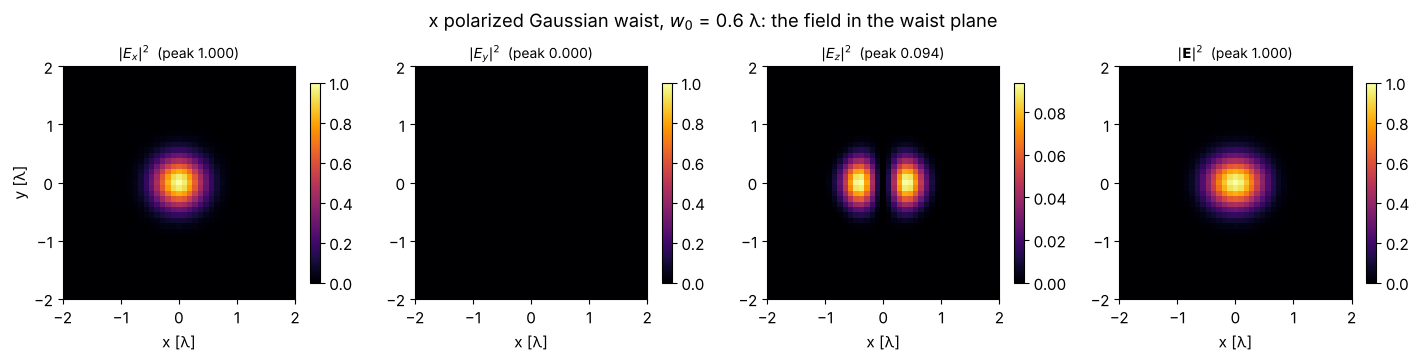
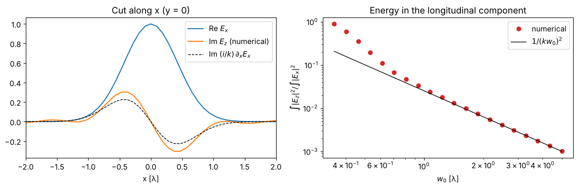
The paraxial estimate fails for waists below about one wavelength: the spectrum then contains plane waves at large angles and evanescent waves, for which \(|E_z| = |E_x|\,|k_x/k_z|\) exceeds \(|E_x|\).

3. Vector beams: radial and azimuthal polarization

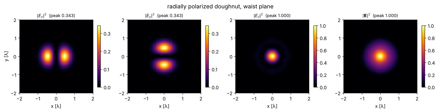
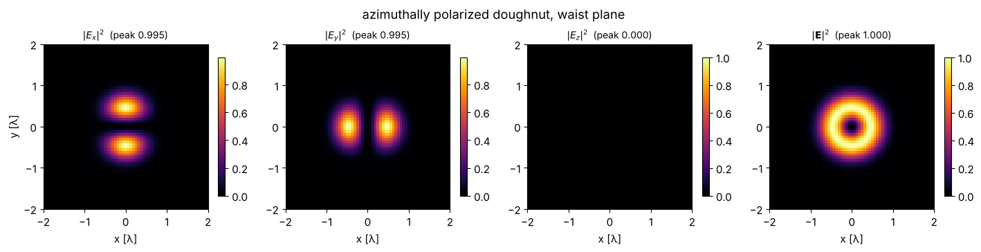
A radially polarized doughnut beam, \([E_x, E_y] = [x, y]\exp(-r^2/w_0^2)\), has a zero of its transverse field on the axis, but its tilted plane waves all have \(E_z\) components of the same sign there: a strong longitudinal field fills the doughnut. The azimuthally polarized beam \([-y, x]\exp(-r^2/w_0^2)\) is divergence free in every plane and has no \(E_z\) at all. We propagate both from their waist (\(w_0 = 0.6\lambda\)) with vectorial_rayleigh_sommerfeld_TF().

Such a tight Gaussian waist contains evanescent waves. Propagating forwards, they decay; propagating backwards (\(z < 0\)) they would grow exponentially, so we keep only the propagating part of the spectrum, \(|\mathbf{k}_\perp| < k\). This is the field a lens could actually produce.

x, y, X, Y = grid(16.0, 256)
w0 = 0.6
G = np.exp(-(X**2 + Y**2)/w0**2)
K_x, K_y = freq_grid(x, y, wavenumbers=True, normal_order=True)
propagating = K_x**2 + K_y**2 < k**2
lowpass = lambda f: inv_FT(FT(f)*propagating)
radial = np.stack([lowpass(X*G), lowpass(Y*G)], -1)
azimuthal = np.stack([lowpass(-Y*G), lowpass(X*G)], -1)

for field, name in ((radial, "radially"), (azimuthal, "azimuthally")):
    E, _, _ = vectorial_rayleigh_sommerfeld_TF(field, x, y, 0.0, wl)
    show_components(E, x, y, "", extent_half=2, fig_title=f"{name} polarized doughnut, waist plane");

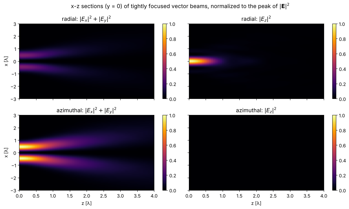
Propagating from the waist plane to \(z = 4\lambda\) shows how the longitudinal on-axis field of the radial beam spreads out; the transverse doughnut keeps its zero on the axis. (We only propagate forwards: going backwards, \(z < 0\), even rounding errors in the evanescent part of the spectrum grow like \(\exp(|k_z||z|)\). For this real waist field \(|\mathbf{E}(-z)| = |\mathbf{E}(z)|\) anyway.)

z_vals = np.linspace(0, 4, 61)
row = 128
xz = {"radial": [], "azimuthal": []}
for z in z_vals:
    for field, name in ((radial, "radial"), (azimuthal, "azimuthal")):
        E, _, _ = vectorial_rayleigh_sommerfeld_TF(field, x, y, z, wl)
        xz[name].append([np.abs(E[row, :, 0])**2 + np.abs(E[row, :, 1])**2, np.abs(E[row, :, 2])**2])
fig, axes = plt.subplots(2, 2, figsize=(12, 7), sharex=True, sharey=True)
for i, name in enumerate(("radial", "azimuthal")):
    data = np.array(xz[name])
    m = data.sum(axis=1).max()
    for j, label in enumerate(("$|E_x|^2 + |E_y|^2$", "$|E_z|^2$")):
        im = axes[i, j].imshow(data[:, j].T/m, extent=[z_vals[0], z_vals[-1], x[0], x[-1]],
                               aspect="auto", cmap="inferno", vmin=0, vmax=1)
        axes[i, j].set_title(f"{name}: {label}")
        axes[i, j].set_ylim(-3, 3)
        fig.colorbar(im, ax=axes[i, j])
for ax in axes[1]:
    ax.set_xlabel("z [λ]")
for ax in axes[:, 0]:
    ax.set_ylabel("x [λ]")
fig.suptitle("x-z sections (y = 0) of tightly focused vector beams, normalized to the peak of $|\\mathbf{E}|^2$")
fig.tight_layout()

4. Any scalar propagator, vectorized: propagate_vectorial()

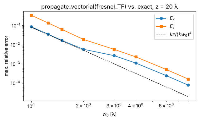
propagate_vectorial() takes a scalar propagator for the transverse components and adds \(E_z\). With rayleigh_sommerfeld_I_TF() (the default inside vectorial_rayleigh_sommerfeld_TF()) the result is exact; with fresnel_TF() it is paraxial. The error of the Fresnel version compared to the exact one, after \(z = 20\lambda\), shrinks with the waist size like the phase error of the Fresnel approximation, \(k z\,\theta^4/8\) with the divergence angle \(\theta \sim 1/(k w_0)\), i.e. like \(w_0^{-4}\):

x, y, X, Y = grid(80.0, 512)
z = 20.0
w0_vals = np.array([1.0, 1.25, 1.5, 2, 3, 4, 6, 8])
errors = {i: [] for i in range(3)}
for w in w0_vals:
    E_x = np.exp(-(X**2 + Y**2)/w**2)
    field = np.stack([E_x, 0*E_x], -1)
    E_exact, _, _ = vectorial_rayleigh_sommerfeld_TF(field, x, y, z, wl)
    E_fr, _, _ = propagate_vectorial(fresnel_TF, field, x, y, z, wl)
    for i in (0, 2):
        errors[i].append(np.abs(E_fr[:, :, i] - E_exact[:, :, i]).max()/np.abs(E_exact[:, :, i]).max())
fig, ax = plt.subplots(figsize=(6.5, 4))
ax.loglog(w0_vals, errors[0], "o-", label="$E_x$")
ax.loglog(w0_vals, errors[2], "s-", label="$E_z$")
ax.loglog(w0_vals, k*z/(k*w0_vals)**4, "k--", lw=1, label="$k z/(k w_0)^4$")
ax.set_xlabel("$w_0$ [λ]"); ax.set_ylabel("max. relative error")
ax.set_title("propagate_vectorial(fresnel_TF) vs. exact, z = 20 λ")
ax.legend(); fig.tight_layout()

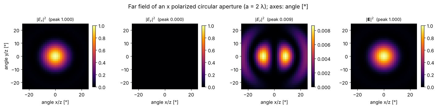
For fraunhofer() (and fresnel_rescaling()) the output grid changes and \(E_z\) follows from the transversality of the far field, \(\mathbf{E}\cdot\mathbf{r} = 0\). Here the far field of a circular aperture of radius \(2\lambda\) illuminated with \(x\) polarized light: the longitudinal component appears in the direction of the polarization, while the transverse components equal the scalar result.

x, y, X, Y = grid(40.0, 256)
a = 2.0
aperture = np.where(X**2 + Y**2 < a**2, 1.0, 0.0)
z_ff = 2000.0
E_ff, x_ff, y_ff = propagate_vectorial(fraunhofer, np.stack([aperture, 0*aperture], -1), x, y, z_ff, wl)
fig = show_components(E_ff, np.degrees(x_ff/z_ff), np.degrees(y_ff/z_ff), "",
                      fig_title="Far field of an x polarized circular aperture (a = 2 λ); axes: angle [°]")
for ax in fig.axes:
    if ax.get_xlabel():
        ax.set_xlabel("angle x/z [°]"); ax.set_xlim(-25, 25); ax.set_ylim(-25, 25)
fig.axes[0].set_ylabel("angle y/z [°]")

Text(129.11284722222223, 0.5, 'angle y/z [°]')

5. Padding vector fields

FFT based propagation is cyclic. propagate_padded() now accepts vector fields; the vectorial propagator computes \(E_z\) inside the padded window. A square aperture (\(6\lambda\), \(x\) polarized) whose spectrum is limited to \(|\mathbf{k}_\perp| < 0.4k\) (as if it were imaged by a lens with NA 0.4) is propagated by \(z = 30\lambda\) in a \(20\lambda\) window. The light diffracted at the largest angles reaches \(|x| \approx 3 + 30\tan(23.6°) \approx 16\lambda\) and wraps around without padding. Note that \(E_z\) lives where the light travels obliquely, i.e. off axis in the \(x\) direction.

x, y, X, Y = grid(20.0, 160)
K_x, K_y = freq_grid(x, y, wavenumbers=True, normal_order=True)
sq = np.where((np.abs(X) < 3) & (np.abs(Y) < 3), 1.0, 0.0)
sq = inv_FT(FT(sq)*(K_x**2 + K_y**2 < (0.4*k)**2))
field = np.stack([sq, 0*sq], -1)
z = 30.0
E_cyc, _, _ = vectorial_rayleigh_sommerfeld_TF(field, x, y, z, wl)
E_pad, _, _ = propagate_padded(vectorial_rayleigh_sommerfeld_TF, field, x, y, z, wl, pad_factor=4)
fig, axes = plt.subplots(1, 5, figsize=(19, 3.6))
ext = [x[0], x[-1], y[0], y[-1]]
for ax, E, c, name in ((axes[0], E_cyc, 0, "$|E_x|^2$, no padding"), (axes[1], E_cyc, 2, "$|E_z|^2$, no padding"),
                       (axes[2], E_pad, 0, "$|E_x|^2$, pad_factor = 4"), (axes[3], E_pad, 2, "$|E_z|^2$, pad_factor = 4")):
    ax.imshow(np.abs(E[:, :, c])**2, extent=ext, cmap="inferno"); ax.set_title(name); ax.set_xlabel("x [λ]")
row = len(y)//2
for E, name, ls in ((E_cyc, "no padding", "--"), (E_pad, "padded", "-")):
    axes[4].plot(x, np.abs(E[row, :, 0])**2, ls, color="C0", label=f"$|E_x|^2$ {name}")
    axes[4].plot(x, 20*np.abs(E[row, :, 2])**2, ls, color="C3", label=f"20 $|E_z|^2$ {name}")
axes[4].set_xlabel("x [λ]"); axes[4].legend(fontsize=8); axes[4].set_title("Cut y = 0")
fig.tight_layout()

6. High NA focusing: Mansuripur’s method

A lens that obeys the sine condition (an aplanatic lens) maps a point \((\rho, \varphi)\) of its pupil, \(\rho = f\sin\theta\), to a plane wave travelling in the direction \(\boldsymbol{\sigma} = (\sin\theta\cos\varphi, \sin\theta\sin\varphi, \cos\theta)\). The polarization of each ray is rotated with the ray about the axis \(\hat{z}\times\boldsymbol{\sigma}\): its s component (perpendicular to the meridional plane) is kept, its p component tilts (aplanatic_rotation()). Energy conservation between the pupil and the converging spherical wave adds the apodization \(1/\sqrt{\cos\theta}\) on the \(\sigma\) grid. This is Mansuripur’s FFT formulation of the Richards-Wolf theory.

vectorial_mansuripur(field, ...) interprets the angular spectrum of field as the pupil. So for a pupil \(P(\sigma_x, \sigma_y)\) we pass inv_FT(P) (the paraxial focal field) and get the vectorial focus at the distance \(z\) from the focal plane.

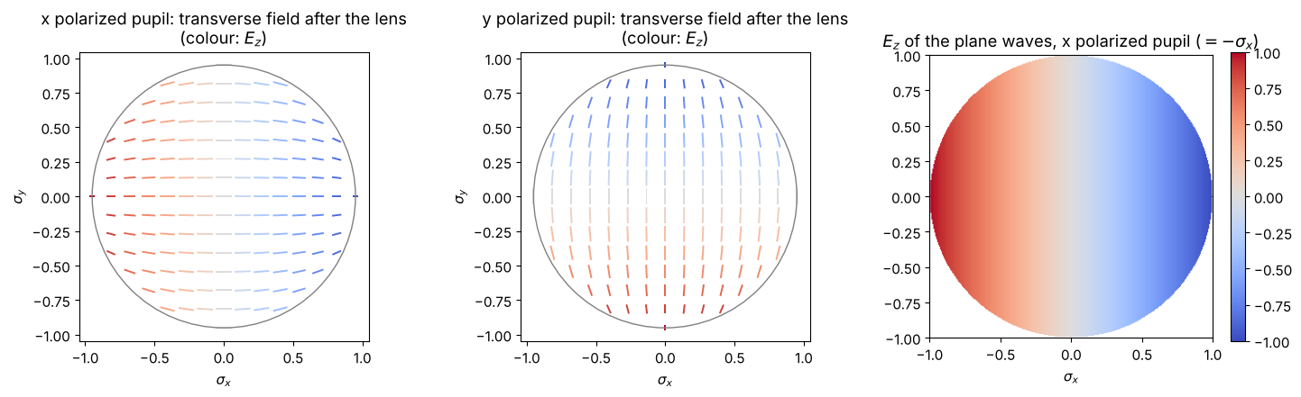
First, the columns of the rotation matrix for an \(x\) polarized pupil: the polarization lines in the pupil after the lens (projected to \(x\)-\(y\)) and the longitudinal part, which is largest along the \(x\) axis.

s = np.linspace(-0.95, 0.95, 15)
SX, SY = np.meshgrid(s, s)
inside = SX**2 + SY**2 <= 0.95**2
R = aplanatic_rotation(np.where(inside, SX, 0), np.where(inside, SY, 0))
fig, axes = plt.subplots(1, 3, figsize=(15, 4.5))
for ax, col, name in ((axes[0], 0, "x"), (axes[1], 1, "y")):
    ax.quiver(SX[inside], SY[inside], R[0, col][inside], R[1, col][inside], R[2, col][inside],
              cmap="coolwarm", pivot="middle", headwidth=1, headlength=0, headaxislength=0, width=0.006, scale=18)
    ax.add_patch(plt.Circle((0, 0), 0.95, fill=False, color="gray"))
    ax.set_aspect("equal"); ax.set_xlabel("$\\sigma_x$"); ax.set_ylabel("$\\sigma_y$")
    ax.set_title(f"{name} polarized pupil: transverse field after the lens\n(colour: $E_z$)")
sg = np.linspace(-1, 1, 301)
SGX, SGY = np.meshgrid(sg, sg)
Rg = aplanatic_rotation(np.clip(SGX, -1, 1)*(SGX**2 + SGY**2 <= 1), SGY*(SGX**2 + SGY**2 <= 1))
im = axes[2].imshow(np.where(SGX**2 + SGY**2 <= 1, Rg[2, 0], np.nan), extent=[-1, 1, -1, 1], cmap="coolwarm", vmin=-1, vmax=1)
axes[2].set_title("$E_z$ of the plane waves, x polarized pupil ($= -\\sigma_x$)")
axes[2].set_xlabel("$\\sigma_x$"); fig.colorbar(im, ax=axes[2])
fig.tight_layout()

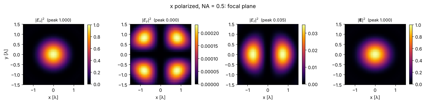
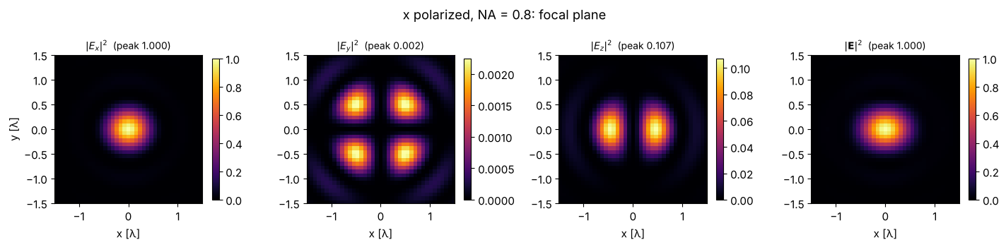
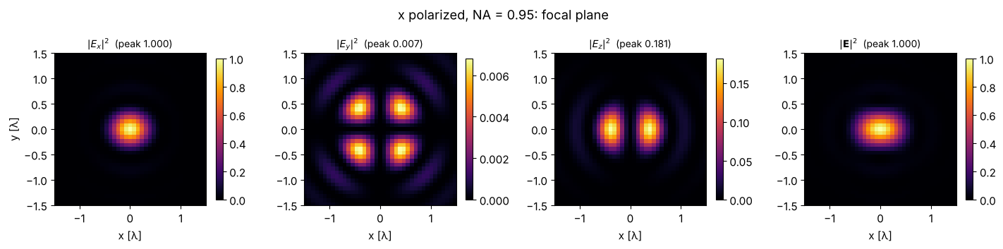
Focal spots for NA 0.5, 0.8 and 0.95

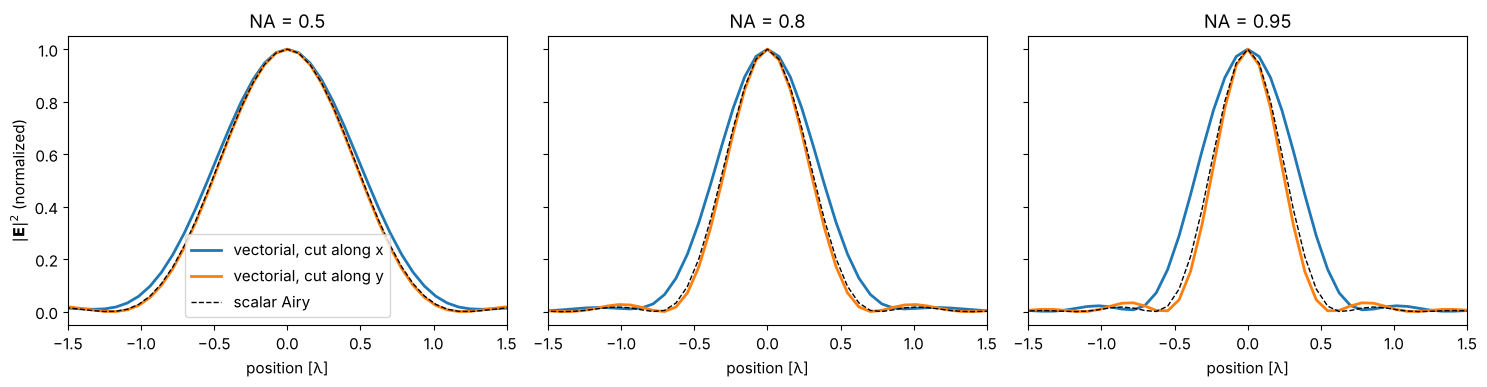
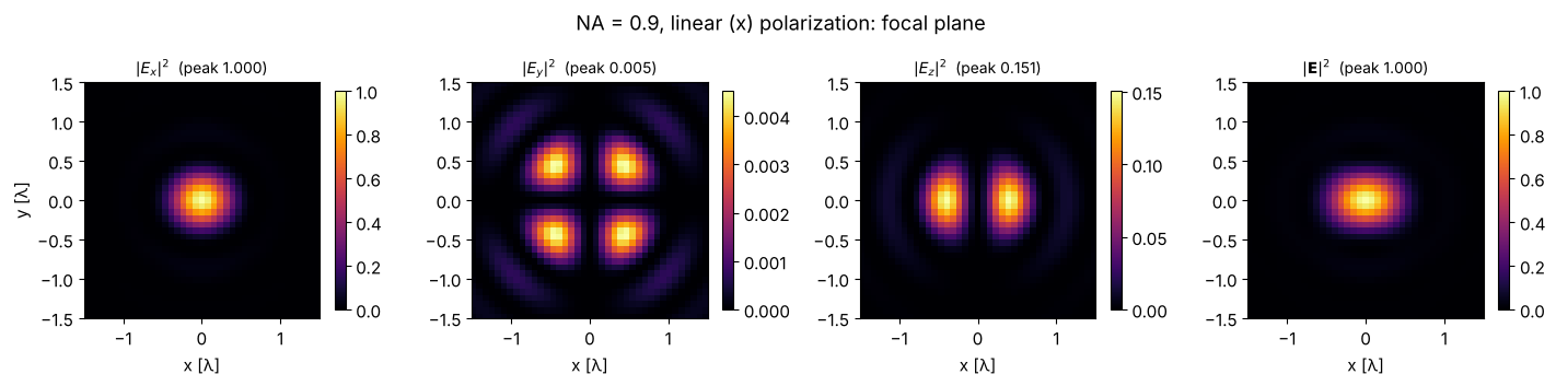
With increasing NA, the \(|E_z|^2\) lobes grow and the total focal spot of linearly polarized light becomes elongated along the polarization direction. The scalar theory (Airy pattern) knows nothing of this.

L, N = 40.0, 512
x, y, X, Y = grid(L, N)
K_x, K_y = freq_grid(x, y, wavenumbers=True, normal_order=True)
S = np.hypot(K_x, K_y)/k
c = N//2

def focus(NA, pol=(1, 0), z=0.0, pupil=None, n=1.0):
    """Vectorial focus of a uniformly filled pupil (or pupil(S) given) with Jones vector pol."""
    P = np.where(S < NA/n, 1.0 if pupil is None else pupil(S), 0.0)
    if callable(pol):
        p_x, p_y = pol(K_x/k, K_y/k)
    else:
        p_x, p_y = pol
    field = np.stack([inv_FT(p_x*P), inv_FT(p_y*P)], -1)
    return vectorial_mansuripur(field, x, y, z, wl, n=n)[0]

for NA in (0.5, 0.8, 0.95):
    E = focus(NA)
    show_components(E, x, y, "", extent_half=1.5, fig_title=f"x polarized, NA = {NA}: focal plane");

Cuts along \(x\) (parallel to the polarization) and \(y\), compared with the scalar Airy pattern \(\left[2J_1(v)/v\right]^2\), \(v = k\,\mathrm{NA}\,r\):

def fwhm(xs, I):
    I = I/I.max()
    i0 = np.argmax(I)
    def side(rng):
        for i in rng:
            if I[i] < 0.5:
                j = i - rng.step
                return xs[i] + (0.5 - I[i])*(xs[j] - xs[i])/(I[j] - I[i])
    return side(range(i0, len(I), 1)) - side(range(i0, -1, -1))

fig, axes = plt.subplots(1, 3, figsize=(15, 4), sharey=True)
xs = x
for ax, NA in zip(axes, (0.5, 0.8, 0.95)):
    E = focus(NA)
    I = sum(components(E)); I /= I.max()
    ax.plot(xs, I[c, :], lw=2, label="vectorial, cut along x")
    ax.plot(xs, I[:, c], lw=2, label="vectorial, cut along y")
    v = k*NA*np.abs(xs) + 1e-12
    ax.plot(xs, (2*j1(v)/v)**2, "k--", lw=1, label="scalar Airy")
    ax.set_xlim(-1.5, 1.5); ax.set_title(f"NA = {NA}"); ax.set_xlabel("position [λ]")
axes[0].set_ylabel("$|\\mathbf{E}|^2$ (normalized)"); axes[0].legend()
fig.tight_layout()

NA_vals = np.linspace(0.2, 0.98, 14)
fw_x, fw_y = [], []
for NA in NA_vals:
    I = sum(components(focus(NA)))
    fw_x.append(fwhm(x, I[c, :])); fw_y.append(fwhm(y, I[:, c]))
fig, axes = plt.subplots(1, 2, figsize=(12, 4))
axes[0].plot(NA_vals, np.array(fw_x)*NA_vals, "o-", label="FWHM along x (polarization)")
axes[0].plot(NA_vals, np.array(fw_y)*NA_vals, "s-", label="FWHM along y")
axes[0].axhline(0.5145, color="k", ls="--", lw=1, label="scalar: 0.514 λ/NA")
axes[0].set_xlabel("NA"); axes[0].set_ylabel("FWHM × NA [λ]"); axes[0].legend()
axes[0].set_title("Spot size in units of λ/NA")
axes[1].plot(NA_vals, np.array(fw_x)/np.array(fw_y), "o-", color="C3")
axes[1].set_xlabel("NA"); axes[1].set_ylabel("FWHM$_x$ / FWHM$_y$"); axes[1].set_title("Ellipticity of the focal spot")
fig.tight_layout()

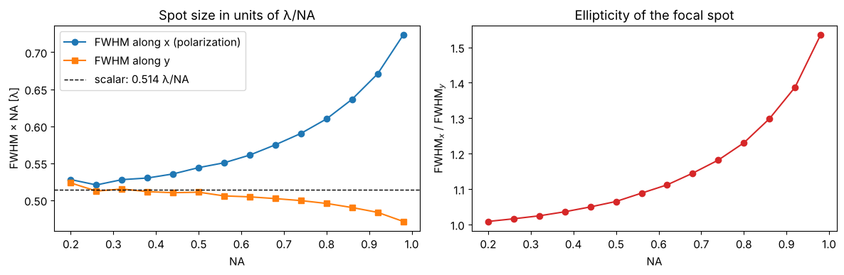
The FWHM is evaluated by linear interpolation on a grid with spacing \(0.078\lambda\), which is good to about 1 %.

Check against the Richards-Wolf integrals

For an \(x\) polarized, uniformly filled pupil Richards and Wolf give the focal field as one-dimensional integrals over the aperture angle \(\theta \le \alpha = \arcsin\mathrm{NA}\):

\[ E_x \propto I_0 + I_2\cos 2\varphi,\quad E_y \propto I_2 \sin 2\varphi,\quad E_z \propto -2i I_1\cos\varphi, \]

\[ I_{0,2} = \int_0^\alpha \sqrt{\cos\theta}\,\sin\theta\,(1\pm\cos\theta)\,J_{0,2}(k\rho\sin\theta)\,e^{ikz\cos\theta}\,d\theta,\quad I_1 = \int_0^\alpha \sqrt{\cos\theta}\,\sin^2\theta\,J_1(k\rho\sin\theta)\,e^{ikz\cos\theta}\,d\theta. \]

We evaluate them with scipy.integrate.quad along the diagonal \(\varphi = 45°\) (where all three components are present) for NA 0.9.

def richards_wolf(rho, phi, z, NA):
    def integral(f):
        g = lambda t: f(t)*np.sqrt(np.cos(t))*np.sin(t)*np.exp(1j*k*z*np.cos(t))
        kw = dict(a=0, b=np.arcsin(NA), limit=200)
        return quad(lambda t: g(t).real, **kw)[0] + 1j*quad(lambda t: g(t).imag, **kw)[0]
    I0 = integral(lambda t: (1 + np.cos(t))*jv(0, k*rho*np.sin(t)))
    I1 = integral(lambda t: np.sin(t)*jv(1, k*rho*np.sin(t)))
    I2 = integral(lambda t: (1 - np.cos(t))*jv(2, k*rho*np.sin(t)))
    return np.array([I0 + I2*np.cos(2*phi), I2*np.sin(2*phi), -2j*I1*np.cos(phi)])

NA = 0.9
fig, axes = plt.subplots(1, 2, figsize=(13, 4))
for ax, z in zip(axes, (0.0, 0.5)):
    E = focus(NA, z=z)
    d = np.arange(0, 14)
    num = np.array([E[c + i, c + i] for i in d])
    rho = np.sqrt(2)*x[c + d]
    ref = np.array([richards_wolf(r, np.pi/4, z, NA) for r in rho])
    scale = np.vdot(ref.ravel(), num.ravel())/np.vdot(ref.ravel(), ref.ravel())
    rr = np.linspace(0, rho[-1], 120)
    ref_fine = np.array([richards_wolf(r, np.pi/4, z, NA) for r in rr])*scale
    m = np.sum(np.abs(num)**2, axis=1).max()
    for i, name in enumerate(("$|E_x|^2$", "$|E_y|^2$", "$|E_z|^2$")):
        ax.plot(rr, np.abs(ref_fine[:, i])**2/m, color=f"C{i}", lw=1.5, label=f"{name} Richards-Wolf")
        ax.plot(rho, np.abs(num[:, i])**2/m, "o", color=f"C{i}", ms=5, label=f"{name} vectorial_mansuripur")
    ax.set_xlabel("ρ along the diagonal [λ]"); ax.set_title(f"NA = {NA}, z = {z} λ")
    print(f"z = {z}: max deviation / peak = {np.abs(num - scale*ref).max()/np.abs(num).max():.1e}")
axes[0].legend(fontsize=8, ncol=2); axes[0].set_ylabel("intensity (normalized)")
fig.tight_layout()

z = 0.0: max deviation / peak = 3.3e-03
z = 0.5: max deviation / peak = 3.7e-03

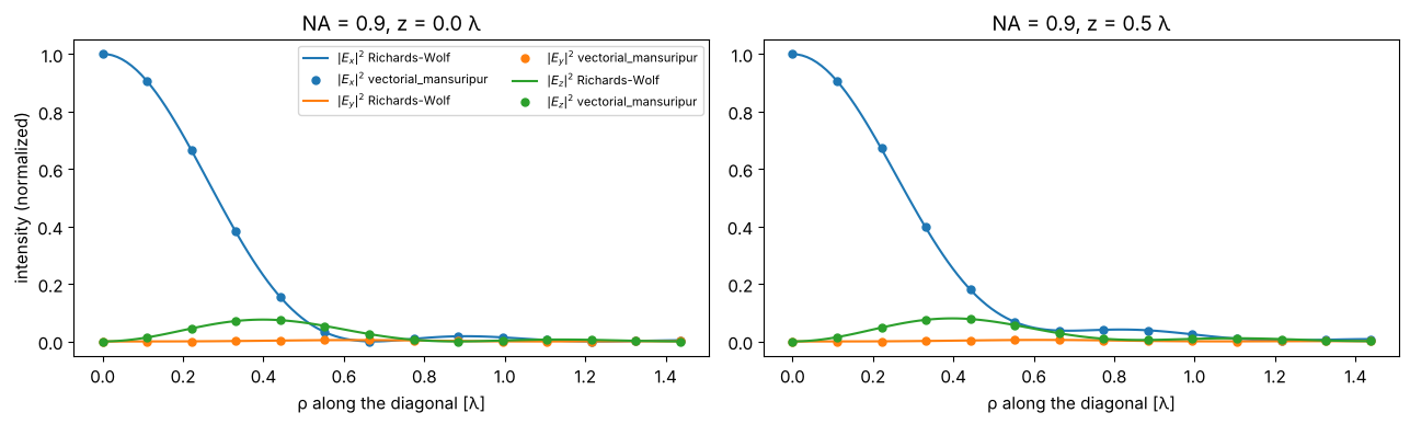
The remaining deviation of a few \(10^{-3}\) comes from sampling the hard pupil edge on the \(\sigma\) grid (\(\Delta\sigma = \lambda/L = 0.025\)). With a smooth pupil the agreement is better than \(10^{-4}\) (see test/test_vectorial.py).

Pupil polarization: linear, circular, radial, azimuthal

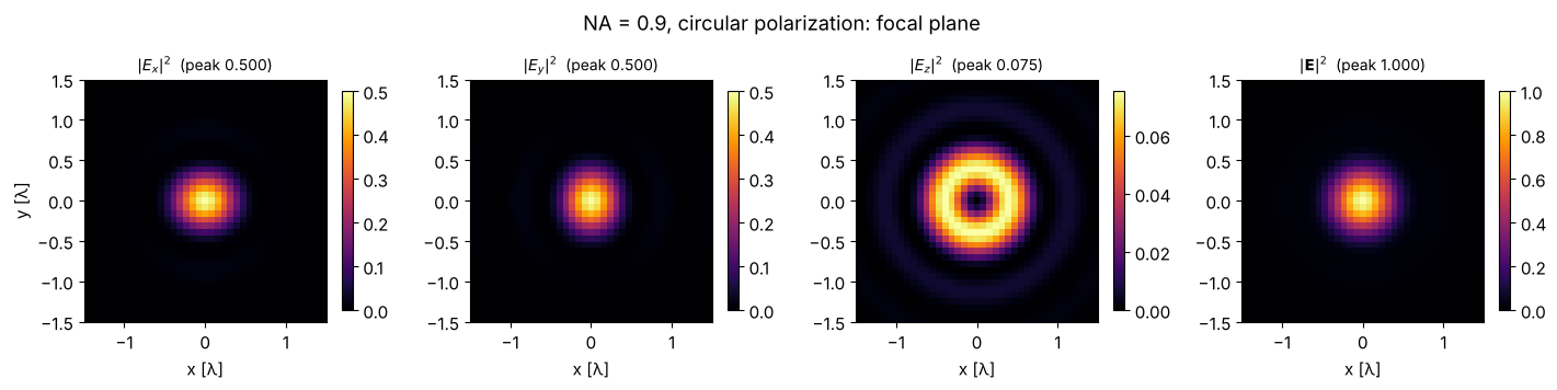
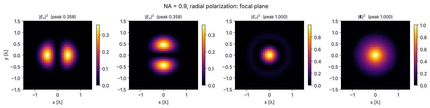
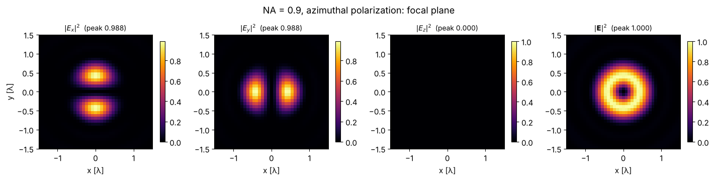
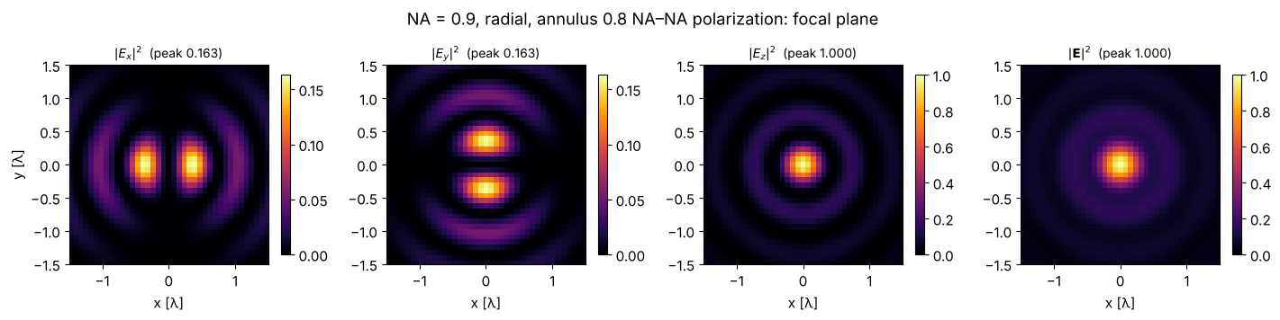
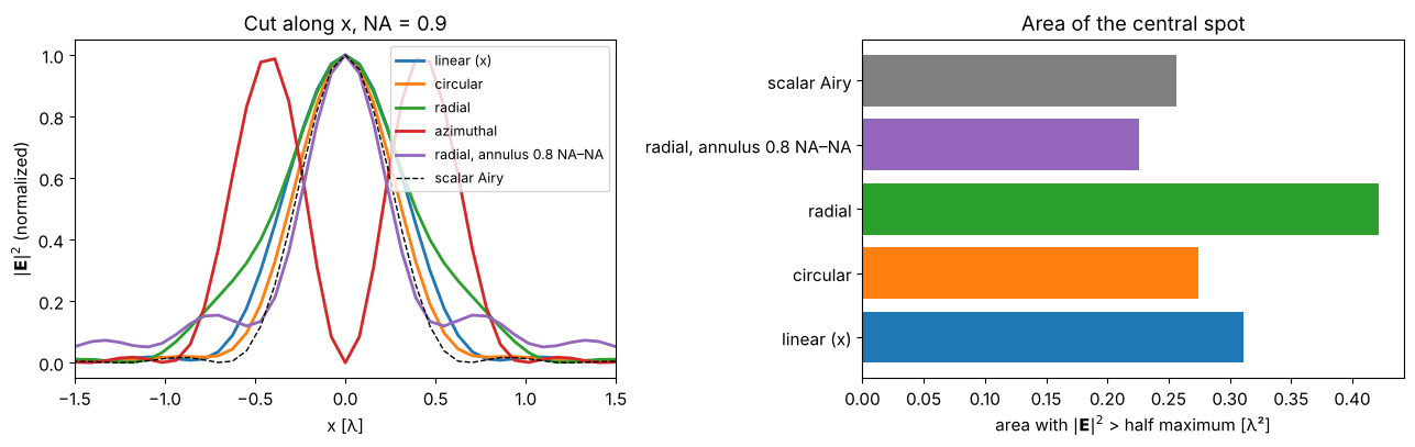
The polarization in the pupil decides the shape of the focus. At NA 0.9:

• linear: elongated spot (see above),

• circular: round spot, but wider than the scalar one, \(E_z\) forms a ring,

• radial: the transverse field has a zero at the center, \(E_z\) a strong peak there,

• azimuthal: no \(E_z\) at all, a doughnut.

Radial polarization with an annular pupil gives a smaller spot than any other polarization, because then the longitudinal component dominates (Quabis et al., Opt. Commun. 179, 1 (2000); Dorn, Quabis and Leuchs, Phys. Rev. Lett. 91, 233901 (2003)).

def radial_pol(sx, sy):
    phi = np.arctan2(sy, sx)
    return np.cos(phi), np.sin(phi)

def azimuthal_pol(sx, sy):
    phi = np.arctan2(sy, sx)
    return -np.sin(phi), np.cos(phi)

NA = 0.9
cases = [("linear (x)", (1, 0), None), ("circular", (1/np.sqrt(2), 1j/np.sqrt(2)), None),
         ("radial", radial_pol, None), ("azimuthal", azimuthal_pol, None),
         ("radial, annulus 0.8 NA–NA", radial_pol, lambda s: (s > 0.8*NA).astype(float))]
results = {}
for name, pol, pupil in cases:
    E = focus(NA, pol=pol, pupil=pupil)
    results[name] = E
    show_components(E, x, y, "", extent_half=1.5, fig_title=f"NA = {NA}, {name} polarization: focal plane");

dA = (x[1] - x[0])**2
fig, axes = plt.subplots(1, 2, figsize=(13, 4.2))
names = list(results)
areas = []
for i, name in enumerate(names):
    I = sum(components(results[name])); I /= I.max()
    axes[0].plot(x, I[c, :], lw=2, label=name)
    areas.append(np.sum(I > 0.5)*dA)
v = k*NA*np.abs(x) + 1e-12
axes[0].plot(x, (2*j1(v)/v)**2, "k--", lw=1, label="scalar Airy")
axes[0].set_xlim(-1.5, 1.5); axes[0].set_xlabel("x [λ]"); axes[0].set_ylabel("$|\\mathbf{E}|^2$ (normalized)")
axes[0].legend(fontsize=9); axes[0].set_title(f"Cut along x, NA = {NA}")
airy_area = np.pi*(0.5145/NA/2)**2
spots = [i for i, name in enumerate(names) if name != "azimuthal"]   # the doughnut has no central spot
axes[1].barh([names[i] for i in spots] + ["scalar Airy"], [areas[i] for i in spots] + [airy_area],
             color=[f"C{i}" for i in spots] + ["gray"])
axes[1].set_xlabel("area with $|\\mathbf{E}|^2$ > half maximum [λ²]")
axes[1].set_title("Area of the central spot")
for i in spots:
    print(f"{names[i]:28s} spot area {areas[i]:.3f} λ²")
print(f"{'scalar Airy':28s} spot area {airy_area:.3f} λ²")
fig.tight_layout()

linear (x)                   spot area 0.311 λ²
circular                     spot area 0.275 λ²
radial                       spot area 0.421 λ²
radial, annulus 0.8 NA–NA    spot area 0.226 λ²
scalar Airy                  spot area 0.257 λ²

Through focus

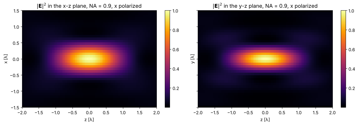
vectorial_mansuripur() takes the distance \(z\) from the focal plane, so a through focus scan is just a loop. \(x\)-\(z\) and \(y\)-\(z\) sections of the total energy density for an \(x\) polarized pupil at NA 0.9: the axial extent is about \(2\lambda/\mathrm{NA}^2\)-ish, the lateral one differs between \(x\) and \(y\).

NA = 0.9
z_vals = np.linspace(-2, 2, 81)
xz, yz = [], []
for z in z_vals:
    I = sum(components(focus(NA, z=z)))
    xz.append(I[c, :]); yz.append(I[:, c])
xz, yz = np.array(xz), np.array(yz)
m = max(xz.max(), yz.max())
fig, axes = plt.subplots(1, 2, figsize=(13, 4.5), sharey=True)
for ax, data, name in ((axes[0], xz, "x"), (axes[1], yz, "y")):
    im = ax.imshow(data.T/m, extent=[z_vals[0], z_vals[-1], x[0], x[-1]], aspect="auto", cmap="inferno")
    ax.set_ylim(-1.5, 1.5); ax.set_xlabel("z [λ]"); ax.set_ylabel(f"{name} [λ]")
    ax.set_title(f"$|\\mathbf{{E}}|^2$ in the {name}-z plane, NA = {NA}, x polarized")
    fig.colorbar(im, ax=ax)
fig.tight_layout()

Energy conservation and transversality

The \(1/\sqrt{\sigma_z}\) weight makes the power flowing through every plane \(z = \mathrm{const}\) equal to the power of the input field, and each plane wave is transverse, so \(\mathbf{k}\cdot\tilde{\mathbf{E}} = 0\):

sz = np.sqrt(np.clip(1 - S**2, 0, None))
for NA in (0.5, 0.9, 0.98):
    P = np.where(S < NA, 1.0, 0.0)
    field = np.stack([inv_FT(P), inv_FT(0*P)], -1)
    p_in = np.sum(np.abs(FT(field[:, :, 0]))**2)
    for z in (0.0, 1.5):
        E = vectorial_mansuripur(field, x, y, z, wl)[0]
        Ek = [FT(E[:, :, i]) for i in range(3)]
        p_out = sum(np.sum(np.abs(Ek[i])**2*sz) for i in range(3))
        div = np.abs(K_x*Ek[0] + K_y*Ek[1] + k*sz*Ek[2]).max()/(k*np.abs(Ek[0]).max())
        print(f"NA {NA}, z = {z}: power out/in = {p_out/p_in:.12f}, max |k·E|/(k max|E|) = {div:.1e}")

NA 0.5, z = 0.0: power out/in = 1.000000000000, max |k·E|/(k max|E|) = 1.4e-15
NA 0.5, z = 1.5: power out/in = 1.000000000000, max |k·E|/(k max|E|) = 1.4e-15

NA 0.9, z = 0.0: power out/in = 1.000000000000, max |k·E|/(k max|E|) = 1.4e-15
NA 0.9, z = 1.5: power out/in = 1.000000000000, max |k·E|/(k max|E|) = 1.3e-15

NA 0.98, z = 0.0: power out/in = 1.000000000000, max |k·E|/(k max|E|) = 1.1e-15
NA 0.98, z = 1.5: power out/in = 1.000000000000, max |k·E|/(k max|E|) = 9.2e-16

Summary

• longitudinal_component() and vectorial_rayleigh_sommerfeld_TF() turn the transverse field in a plane into the full, divergence free vector field in any other plane, exactly.

• propagate_vectorial() does the same for every scalar propagator, so Fresnel and Fraunhofer computations get their \(E_z\) too; propagate_padded() pads vector fields.

• vectorial_mansuripur() (formerly vectorial_fresnel(), which is now a deprecated alias) computes the focus of an aplanatic lens and agrees with the Richards-Wolf integrals. Linearly polarized foci are elongated along the polarization; radial polarization with an annular pupil gives the smallest spot.

References

• B. Richards and E. Wolf, “Electromagnetic diffraction in optical systems II. Structure of the image field in an aplanatic system”, Proc. R. Soc. Lond. A 253, 358-379 (1959).

• M. Mansuripur, “Distribution of light at and near the focus of high-numerical-aperture objectives”, J. Opt. Soc. Am. A 3, 2086-2093 (1986).

• M. Mansuripur, “Certain computational aspects of vector diffraction problems”, J. Opt. Soc. Am. A 6, 786-805 (1989), erratum J. Opt. Soc. Am. A 10, 382 (1993).

• L. Novotny and B. Hecht, Principles of Nano-Optics, 2nd ed., Cambridge University Press (2012).

• K. S. Youngworth and T. G. Brown, “Focusing of high numerical aperture cylindrical-vector beams”, Opt. Express 7, 77-87 (2000).

• S. Quabis, R. Dorn, M. Eberler, O. Glöckl and G. Leuchs, “Focusing light to a tighter spot”, Opt. Commun. 179, 1-7 (2000).

• R. Dorn, S. Quabis and G. Leuchs, “Sharper focus for a radially polarized light beam”, Phys. Rev. Lett. 91, 233901 (2003).