Delano diagrams: first order layout of a lithography lens

Delano’s \(y\)-\(\bar y\) diagram plots the height \(\bar y\) of the paraxial chief ray against the height \(y\) of the paraxial marginal ray at every lens (or surface). A system becomes a polygon, and all of its first order properties can be read off it: powers, spacings, stop and pupils, telecentricity, conjugates, cardinal points. The other way round, a lens can be drawn as a polygon and then built from it. This is how complex systems such as lithographic projection lenses are laid out before any surface is bent (Delano 1963; Shack 1973; Matsuyama, Ohmura and Williamson, “The lithographic lens: its history and evolution”, Proc. SPIE 6154, 2006).

This notebook

1. reads the diagram of Caldwell’s KrF lens (DelanoDiagram.from_system()),

2. shows the rules of the diagram with a three lens relay,

3. lays out a new KrF projection lens in the diagram: 20 elements, 1 m from object to wafer, magnification −0.25, NA 0.7, telecentric on both sides, with a flat field (Petzval sum zero) — first as a hand drawn sketch, then polished with delano.refine(),

4. turns the thin lens layout into fused silica singlets with the same first order properties (delano.thicken()),

5. corrects the aberrations with real rays (lens_optimization.LensOptimizer, five aspheric surfaces, all lenses at least 10 mm thick at the centre and the edge) and checks the result.

Conventions (module pyoptics.delano): points \(P = (\bar y, y)\), reduced slopes \(\omega = n u\), Lagrange invariant \(H = n(\bar u y - u \bar y)\), as raytrace.Paraxial.lagrange. Lengths in mm.

import time

import numpy as np
import matplotlib.pyplot as plt

from pyoptics import raytrace as rt
from pyoptics import lens_optimization as lo
from pyoptics.delano import DelanoDiagram, refine, thicken

plt.rcParams.update({"figure.dpi": 80, "font.size": 11})
t_start = time.time()

1. The diagram of a real lens

DelanoDiagram.from_system() takes the paraxial marginal and chief rays of a raytrace.System: one point per surface vertex, plus the object and the image point. Caldwell’s all fused silica KrF lens (21 elements, NA 0.56, 4x, 1 m) as an example:

caldwell = rt.caldwell_krf_lens()
dc = DelanoDiagram.from_system(caldwell)
p = caldwell.paraxial()

fig, axes = plt.subplots(1, 2, figsize=(16, 5.2), gridspec_kw={"width_ratios": [1.2, 1]})
caldwell.draw(axes[0], fields=[0.0, caldwell.max_field])
axes[0].set_title("Caldwell's KrF lens: 21 elements, NA 0.56, 4x")
dc.plot(axes[1], annotate=False, areas=True)
for k in [0, 1, 11, 23, 30, 37, 41, 43]:
    axes[1].annotate(dc.labels[k], (dc.ybar[k], dc.y[k]), xytext=(4, 4), textcoords="offset points",
                     fontsize=8)
axes[1].set_title("its y-ȳ diagram, one point per surface")
fig.tight_layout()

n_s = caldwell.n*caldwell.sigma
powers = np.array([s.paraxial_power(n_s[i], n_s[i + 1]) for i, s in enumerate(caldwell.surfaces)])
print(f"{len(dc)} points: object, 42 surfaces, image; H = {dc.H:.4f} mm")
print(f"powers from the corners vs. (n' - n)/R: max. difference {np.max(abs(dc.power - powers)):.1e} 1/mm")
print(f"spaces from the triangle areas vs. the thicknesses: max. difference "
      f"{np.max(abs(dc.thickness[1:-1] - [s.thickness for s in caldwell.surfaces[:-1]])):.1e} mm")
print(f"magnification {dc.magnification:.5f} (paraxial {p.magnification:.5f}), "
      f"NA {dc.NA[1]:.4f} (paraxial {p.na:.4f}), length {dc.length:.2f} mm")
pu = dc.pupils()
print(f"stop (y axis crossing) {pu.stop[0]:.1f} mm behind the object, surface 30 at "
      f"{caldwell.object_distance + caldwell.vertex_z[29]:.1f} mm; entrance pupil "
      f"{pu.entrance/1e3:.1f} m, exit pupil {pu.exit/1e3:.1f} m from the object")

44 points: object, 42 surfaces, image; H = -6.2702 mm
powers from the corners vs. (n' - n)/R: max. difference 1.3e-16 1/mm
spaces from the triangle areas vs. the thicknesses: max. difference 7.5e-14 mm
magnification -0.25000 (paraxial -0.25000), NA 0.5359 (paraxial 0.5359), length 1000.01 mm
stop (y axis crossing) 701.8 mm behind the object, surface 30 at 701.8 mm; entrance pupil 10.0 m, exit pupil -2.6 m from the object

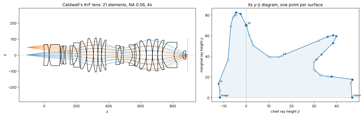
How to read it:

• The polygon starts at the object on the \(\bar y\) axis (\(y = 0\), \(\bar y\) = object height 46.8 mm) and ends at the image (\(\bar y = -11.7\) mm). It crosses the \(y\) axis (\(\bar y = 0\)) once, at the aperture stop (star), here at surface 30.

• The first and the last edges are almost vertical: the chief ray is almost parallel to the axis in object and image space, the lens is (nearly) telecentric on both sides. The extended edges meet \(\bar y = 0\) at the pupils, 9 m in front of and 2.6 m behind the lens.

• Every edge is a space: the shaded triangle that it spans with the origin has the area \(H\tau/2\), with the reduced thickness \(\tau = t/n\). Long air spaces far from the origin are large triangles; a glass element is two corners close together.

• Every corner is a surface: its power is the change of direction, \(\phi_k = -(\bar\omega_{k-1}\omega_k - \omega_{k-1}\bar\omega_k)/H\). A convex corner (turning towards the origin) is positive (filled circles), a concave one negative (open circles). The same bend is a weak surface far from the origin and a strong one close to it.

• The shape is the classic one of lithography lenses: bulges (large beams, positive groups) and waists (small beams, negative groups) alternate. The waists correct the Petzval sum: the Petzval sum of thin lenses \(\sum \phi_k/n_k\) does not depend on where a lens sits, but its contribution to the imaging, the bend of the marginal ray \(y_k\phi_k\), does. Negative lenses in a waist (small \(y\)) flatten the field at little cost in power.

2. The rules, with three thin lenses

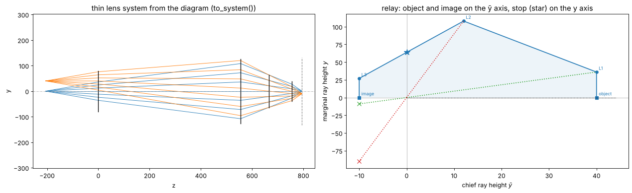
A double telecentric 4x relay of three thin lenses, drawn directly as a polygon: object \((h, 0)\), a vertical edge up (telecentric object space), a corner at the top, down to \((-h/4, y_3)\) and vertically down to the image \((-h/4, 0)\). The Lagrange invariant follows from the object side NA, \(H = -\mathrm{NA}_\mathrm{obj}\,h\); with_length() scales all \(y\) so that the system is 1 m long (same NA, field and magnification).

h = 40.0
relay = DelanoDiagram([h, h, 0.3*h, -0.25*h, -0.25*h], [0, 20, 60, 15, 0], -0.175*h,
                      labels=["object", "L1", "L2", "L3", "image"]).with_length(1000.0)
relay_system = relay.to_system(248.3e-6)
pr = relay_system.paraxial()
print("focal lengths", np.round(relay.focal_length, 1), "mm; spaces", np.round(relay.thickness, 1), "mm")
print(f"thin lens system: magnification {pr.magnification:.4f}, NA {pr.na:.4f}, "
      f"length {relay_system.object_distance + relay_system.image_z:.1f} mm, "
      f"entrance/exit pupil at {pr.ep_z:.1e}/{pr.xp_z:.1e} mm (telecentric)")

fig, axes = plt.subplots(1, 2, figsize=(16, 5))
relay_system.draw(axes[0], fields=[0.0, h])
axes[0].set_title("thin lens system from the diagram (to_system())")
relay.plot(axes[1], areas=True)
# conjugates lie on lines through the origin
axes[1].plot([0, 1.1*h], [0, 0], "k:", lw=1)
z_stop = relay.pupils().stop[0]
for k, c in [(1, "C2"), (2, "C3")]:
    z, m = relay.conjugate(3, k)
    q = m*relay.points[k]
    axes[1].plot([0, relay.ybar[k]], [0, relay.y[k]], ":", color=c)
    axes[1].plot([0, q[0]], [0, q[1]], ":", color=c)
    axes[1].plot(*q, "x", color=c, ms=8)
    print(f"image of {relay.labels[k]} in the last space: z = {z:.1f} mm, magnification {m:.3f}")
axes[1].set_title("relay: object and image on the ȳ axis, stop (star) on the y axis")
fig.tight_layout()

focal lengths [793.2 202.4  91.1] mm; spaces [205.7 555.3 200.5  38.6] mm
thin lens system: magnification -0.2500, NA 0.7000, length 1000.0 mm, entrance/exit pupil at inf/-4.1e+17 mm (telecentric)
image of L1 in the last space: z = 1012.9 mm, magnification -0.250
image of L2 in the last space: z = 1128.5 mm, magnification -0.833

3. Specification and sketch of the new lens

The specification fixes the ends of the polygon:

	in the diagram
magnification −0.25	object at \((h, 0)\), image at \((-h/4, 0)\)
telecentric object and image space	first and last edges vertical: \(\bar y_1 = h\), \(\bar y_{20} = -h/4\)
NA 0.7 (object side 0.175)	\(H = -0.175\,h\); the slopes of the first and last edges follow
1 m object to wafer	scale all \(y\) (with_length())
image field radius 13.6 mm (a 26 × 8 mm scanner slit)	\(h = 54.4\) mm
flat field	Petzval sum \(\sum\phi_k/n = 0\)

Everything in between is design. Rules for drawing the polygon:

• It has to wind around the origin in one sense (here counterclockwise): a step back in angle would be a negative distance.

• Distances are areas: a lens close to the origin gets little room.

• The last space is the working distance (more precisely, from the rear principal plane of the last lens to the wafer): \(t = y_{20}/\mathrm{NA}\).

• Lenses carry diameters \(2(|y| + |\bar y|)\); with 1 m length and NA 0.7 the largest are about 250 mm.

The sketch below has the structure of the lens of section 1 with fewer elements: three positive field lenses (L1–L3, telecentric object space), a first waist of three negative lenses (L4–L6), a bulge (L7–L10), a second waist (L11–L13), and the last bulge with the stop (L14–L20), which does most of the focusing to NA 0.7. It is written in units of \(h\) for \(\bar y\) and of an arbitrary scale for \(y\) (with_length() fixes it).

WL = 248.3e-6                     # KrF, mm
N_SIO2 = rt.fused_silica(248.3)
M, LENGTH, NA = -0.25, 1000.0, 0.7
R_FIELD = 13.6                    # image field radius
h = R_FIELD/abs(M)                # object height
H = -NA*abs(M)*h                  # Lagrange invariant

# (ybar/h, y) of object, L1...L20, image
SKETCH = np.array([(1, 0), (1, 0.08), (0.97, 0.15), (0.92, 0.21), (0.82, 0.21), (0.74, 0.20),
                   (0.66, 0.22), (0.60, 0.33), (0.52, 0.47), (0.42, 0.57), (0.32, 0.61),
                   (0.24, 0.53), (0.18, 0.46), (0.12, 0.45), (0.07, 0.58), (0.02, 0.74),
                   (-0.04, 0.86), (-0.10, 0.88), (-0.16, 0.74), (-0.21, 0.48), (-0.25, 0.10),
                   (-0.25, 0)])
labels = ["object"] + [f"L{k}" for k in range(1, 21)] + ["image"]
sketch = DelanoDiagram(h*SKETCH[:, 0], SKETCH[:, 1], H, labels=labels).with_length(LENGTH)


def summary(d, name):
    print(f"{name}: Petzval sum {d.petzval_sum(N_SIO2)*1e3:+.3f}/m, NA {d.NA[0]:.3f} -> {d.NA[1]:.3f}, "
          f"magnification {d.magnification:.3f}, length {d.length:.1f} mm, stop at "
          f"{d.pupils().stop[0]:.0f} mm")
    print("  f    [mm]", " ".join(f"{f:6.0f}" for f in d.focal_length))
    print("  space[mm]", " ".join(f"{t:6.1f}" for t in d.thickness))
    print("  y*phi[%] ", " ".join(f"{v:6.1f}" for v in 100*d.y[1:-1]*d.power))
    print("  semi diam", " ".join(f"{v:6.1f}" for v in d.heights()[1:-1]))


summary(sketch, "sketch")

sketch: Petzval sum +1.437/m, NA 0.175 -> 0.700, magnification -0.250, length 1000.0 mm, stop at 696 mm
  f    [mm]   2086   2419    199    156    -95   -301  20471   1575   1053    132    376    -93   -102   -883    452    343    306    528    782    535
  space[mm]   69.2   62.6   56.8   18.2    7.4   26.6   74.2   95.4   85.6   63.8   20.1   13.0   22.3   32.9   34.8   40.5   43.9   57.7   67.9   85.6   21.6
  y*phi[%]     0.6    0.9   16.0   20.3  -31.7  -11.1    0.2    4.5    8.2   69.8   21.3  -74.9  -66.5   -9.9   24.8   38.0   43.6   21.2    9.3    2.8
  semi diam   66.5   75.5   81.8   76.4   70.5   69.2   82.6   99.4  109.1  109.7   93.2   79.4   74.6   91.6  113.0  132.3  138.6  120.7   84.0   28.7

The sketch already has the intended signs and a small Petzval sum (a Petzval radius of about 0.7 m). Its weak points are in the row “y*phi”, the bend \(y_k\phi_k\) of the marginal ray at each lens (the whole lens bends it by 0.875, from +0.175 to −0.7): L10 at the corner into the second waist and L12, L13 in it bend it by about ±0.7 each and cancel, which costs aberrations, while L1, L2 and L7 do almost nothing; and the spaces around L5 and L12 are too short for real lenses.

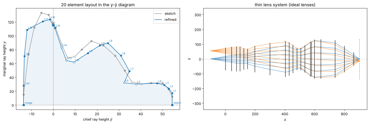
refine() moves the points of the sketch (keeping the telecentric ends) to a Petzval sum of zero, spaces of at least 25 mm, a working space of 40 mm, semi diameters up to 125 mm and the signs of the sketch, while staying close to it and spreading the bending of the marginal ray over the lenses. It is a small least squares problem in the 38 free coordinates of the inner points (seconds).

layout = refine(sketch, N_SIO2, min_space=25.0, spaces={-1: 40.0}, max_height=125.0, anchor=1.0)
summary(layout, "refined")

fig, axes = plt.subplots(1, 2, figsize=(16, 5.5))
sketch.plot(axes[0], color="0.6", label="sketch", annotate=False)
layout.plot(axes[0], color="C0", label="refined", areas=True)
axes[0].legend()
axes[0].set_title("20 element layout in the y-ȳ diagram")
thin = layout.to_system(WL)
thin.draw(axes[1], fields=[0.0, h])
axes[1].set_title("thin lens system (ideal lenses)")
fig.tight_layout()
pt = thin.paraxial()
print(f"thin lens system: m = {pt.magnification:.5f}, NA = {pt.na:.4f}, "
      f"length = {thin.object_distance + thin.image_z:.2f} mm, telecentric: "
      f"pupils at {pt.ep_z:.1e} and {pt.xp_z:.1e} mm")

refined: Petzval sum +0.000/m, NA 0.175 -> 0.700, magnification -0.250, length 1000.0 mm, stop at 677 mm
  f    [mm]   1445   2018    727    188   -223   -123    403   1657    275    290   6282   -109   -110  -1219    331    251   2050    223    925   2354
  space[mm]   98.2   41.8   31.6   25.0   25.0   25.0   49.6  101.3  103.8   25.0   25.0   28.3   25.0   27.0   36.9   28.6   42.4   96.8   61.8   62.1   40.0
  y*phi[%]     1.2    1.2    4.0   16.8  -13.5  -26.2   12.2    4.3   32.6   29.6    1.2  -56.6  -58.5   -6.8   33.6   49.2    5.9   48.6    7.6    1.2
  semi diam   71.6   76.8   79.6   79.0   68.0   64.6   83.9  102.2  114.6  107.1   90.5   71.2   70.4   86.9  112.0  125.0  125.5  120.5   84.0   41.6
thin lens system: m = -0.25000, NA = 0.7000, length = 1000.00 mm, telecentric: pupils at -1.1e+18 and -1.2e+18 mm

4. Thick lenses with the same first order properties

thicken() replaces every thin lens by a fused silica singlet of the same power, with a centre thickness (here 0.2 × the paraxial semi diameter, 15–40 mm, the last lens 30 mm) and a shape factor \(X = (c_1 + c_2)/(c_1 - c_2)\) (here equiconvex/equiconcave, \(X = 0\)). The principal planes of each singlet sit where the thin lens was, so the paraxial rays in all air spaces stay those of the layout; only the distance between the principal planes of each lens adds to the length, which length= takes out by rescaling the diagram. The diagram of the thick system (one point per surface) goes through the same lines as the thin one:

T = np.clip(0.2*layout.heights()[1:-1], 15, 40)
T[-1] = 30.0
start = thicken(layout, WL, rt.fused_silica, T, 0.0, length=LENGTH, check=False)
d_start = DelanoDiagram.from_system(start)
ps = start.paraxial()
print(f"thick start system: m = {ps.magnification:.5f}, NA = {ps.na:.4f}, "
      f"length = {start.object_distance + start.image_z:.2f} mm")
sd = start.seidel()
print(f"Seidel sums at full field: W040 = {sd.W040:.0f}, W131 = {sd.W131:.0f}, W222 = {sd.W222:.0f}, "
      f"W220 = {sd.W220:.0f}, W311 = {sd.W311:.0f} waves")

fig, axes = plt.subplots(1, 2, figsize=(16, 5.5))
layout.with_length(LENGTH).plot(axes[0], color="0.6", label="thin layout", annotate=False)
d_start.plot(axes[0], color="C1", label="thick singlets (surfaces)", annotate=False, signs=False)
axes[0].legend()
axes[0].set_title("thin and thick: the same polygon outside the glass")
start.draw(axes[1], fields=[0.0, h])
axes[1].set_title("start system: equiconvex/equiconcave singlets")
fig.tight_layout()

thick start system: m = -0.25000, NA = 0.7000, length = 1000.00 mm
Seidel sums at full field: W040 = -32503, W131 = 15709, W222 = -664, W220 = -411, W311 = 725 waves

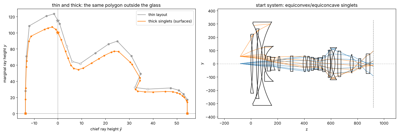
First order is now right, third order not at all: the lenses are not bent yet, the spherical aberration alone is thousands of waves.

5. Correcting the aberrations with real rays

LensOptimizer varies all curvatures, all thicknesses (glass and air), the object distance and the \(r^4\), \(r^6\) and \(r^8\) coefficients of five aspheric surfaces, about evenly spread from the reticle to the wafer (the rear of L2, the front of L6, the rear of L10, the front of L15 next to the stop, the rear of L19), and minimizes, by damped least squares, the residuals of

• the transverse ray errors relative to the chief ray on four rings of the pupil at six fields (tolerance 0.1 µm),

• distortion against \(m = -0.25\) at five fields (10 nm), image and object side telecentricity, the paraxial magnification,

• clearances: centre and edge thicknesses of at least 10 mm, air spaces of 1 mm, 30 mm in front of the reticle, 8 mm working distance, checked at the rim of the full beam.

The length stays 1 m (the image distance is solved) and the object side NA 0.175 (the stop size is solved). A local optimizer cannot open a lens from scratch to NA 0.7 and the full field, the rays at the rim of the pupil fail (they miss surfaces or are totally reflected). As in end-to-end lens design by gradient descent, the aperture and the field are opened in stages, here in three phases:

1. 40 %, 60 %, 80 % and 90 % of the NA and the field, telecentricity to 1 mrad;

2. 90 % to 100 % in small steps (a large last step loses the rim rays of the full field), telecentricity to 0.2 mrad;

3. at full aperture and field, telecentricity and distortion of the real chief ray (aim=True). The ray traces of the optimizer aim at the paraxial entrance pupil (no ray aiming, 20 times faster), and at NA 0.7 the pupil aberrations put the ray that starts towards it tens of mrad away from the ray through the centre of the stop; aim=True aims the chief ray alone at the stop.

The full run takes about two and a half hours; it is reproduced in the cell below with RUN_FULL = True. Otherwise only a few steps of the first stage run here and the result of the full run is loaded from raytrace.delano_krf_lens(), which stores it.

RUN_FULL = False


def operands(telecentricity, aim):
    return [lo.ray_errors(fields=(0, 0.35, 0.6, 0.8, 0.9, 1), tolerance=1e-4),
            lo.distortion(M, fields=(0.25, 0.5, 0.7, 0.85, 1), aim=aim),
            lo.image_telecentricity(tolerance=telecentricity, aim=aim),
            lo.object_telecentricity(tolerance=telecentricity, aim=aim),
            lo.paraxial_target("magnification", M, 1e-5),
            lo.clearances(min_center=10.0, min_edge=10.0, min_image_distance=8.0,
                          min_object_distance=30.0)]


lens_surfaces = [i for i in range(len(start.surfaces)) if start.n[i] != start.n[i + 1]]
ASPHERES = [lens_surfaces[2*k + j] for k, j in [(1, 1), (5, 0), (9, 1), (14, 0), (18, 1)]]
phases = [(operands(1e-3, False), [(a, a) for a in (0.4, 0.6, 0.8, 0.9)], 150),
          (operands(2e-4, False), [(a, a) for a in (0.9, 0.94, 0.97, 1.0)], 200),
          (operands(2e-4, True), [(1.0, 1.0)]*3, 150)]
start.ray_aiming = False  # paraxial pupil aiming is much faster
t0 = time.time()
system, log = start, []
for ops, stages, nfev in (phases if RUN_FULL else [(phases[0][0], phases[0][1][:1], 5)]):
    opt = lo.LensOptimizer(system, ops, thicknesses=list(range(len(system.surfaces) - 1)),
                           object_distance=True, length=LENGTH, object_na=NA*abs(M),
                           aspheres=ASPHERES, asphere_orders=(4, 6, 8))
    result = opt.run(stages=stages, max_nfev=nfev)
    system = result.system
    log += result.stages
design = system if RUN_FULL else rt.delano_krf_lens()
print(f"aspheres on surfaces {[i + 1 for i in ASPHERES]}; {len(opt.x)} variables, "
      f"{len(opt.residuals())} residuals, {time.time() - t0:.0f} s")
for na_f, field_f, cost, nfev in log:
    print(f"  stage at {na_f:.0%} NA, {field_f:.0%} field: cost {cost:.4g} after {nfev} evaluations")

aspheres on surfaces [4, 11, 20, 29, 39]; 96 variables, 308 residuals, 16 s
  stage at 40% NA, 40% field: cost 8.194e+09 after 5 evaluations

6. The corrected lens

design.ray_aiming = True
pd = design.paraxial()
d_design = DelanoDiagram.from_system(design)
glass = [i for i in range(len(design.surfaces)) if not design._is_gap(design.n[i + 1])]
print(f"design: m = {pd.magnification:.5f}, NA = {pd.na:.4f}, "
      f"length = {design.object_distance + design.image_z:.3f} mm, working distance "
      f"{design.surfaces[-1].thickness:.1f} mm, object distance {design.object_distance:.1f} mm, "
      f"{sum(design.surfaces[i].thickness for i in glass):.0f} mm of glass, "
      f"largest semi diameter {np.max(d_design.heights()):.0f} mm")
edge = lo.clearances(min_center=10.0, min_edge=10.0, margin=1.0, tolerance=1.0)(design)
print(f"thinnest centre {min(design.surfaces[i].thickness for i in glass):.1f} mm, "
      f"largest clearance violation {np.max(edge):.2f} mm")

fig, axes = plt.subplots(1, 2, figsize=(16, 5.5), gridspec_kw={"width_ratios": [1.2, 1]})
design.draw(axes[0], fields=[0.0, 0.7*h, h])
axes[0].set_title("corrected 20 element lens, 5 aspheres, NA 0.7, 4x")
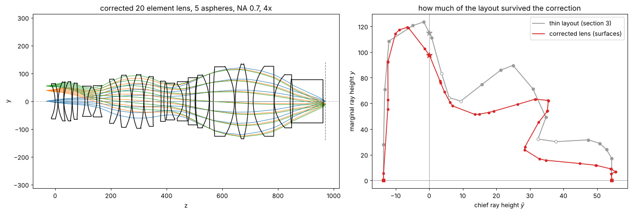
layout.plot(axes[1], color="0.6", label="thin layout (section 3)", annotate=False)
d_design.plot(axes[1], color="C3", label="corrected lens (surfaces)", annotate=False, signs=False)
axes[1].legend()
axes[1].set_title("how much of the layout survived the correction")
fig.tight_layout()

design: m = -0.25000, NA = 0.7000, length = 1000.000 mm, working distance 8.0 mm, object distance 30.0 mm, 699 mm of glass, largest semi diameter 126 mm
thinnest centre 10.0 mm, largest clearance violation 0.00 mm

fields = np.linspace(0, 1, 11)
rms = np.array([design.rms_opd(field=f*h, N=48) for f in fields])
spots = [design.spot_diagram(f*h, N=21) for f in fields]
dist, tele, tele_obj = [], [], []
for f in fields:
    rays = design.rays(f*h, 0.0, 0.0)  # the chief ray, aimed at the centre of the stop
    d0 = np.reshape(rays.directions, (-1, 3))[0]
    I, D = design._image_hits(design.trace(rays, clip=False))
    dist.append((I[0, 1] - M*f*h)*1e6)
    tele.append(D[0, 1]/D[0, 2]*1e3)
    tele_obj.append(d0[1]/d0[2]*1e3)

fig, axes = plt.subplots(1, 3, figsize=(17, 4.2))
r_img = fields*R_FIELD
axes[0].plot(r_img, rms, "o-", label="RMS wavefront error")
axes[0].axhline(0.07, color="k", ls="--", lw=0.8, label="Maréchal limit λ/14")
axes[0].set_xlabel("image field radius [mm]"); axes[0].set_ylabel("waves")
axes[0].set_ylim(0, None); axes[0].legend(fontsize=9); axes[0].set_title("wavefront error")
axes[1].plot(r_img, [s.rms*1e3 for s in spots], "o-", label="RMS spot radius")
axes[1].axhline(0.61*WL*1e3/NA, color="k", ls="--", lw=0.8, label="Airy radius 0.61 λ/NA")
axes[1].set_xlabel("image field radius [mm]"); axes[1].set_ylabel("µm"); axes[1].legend(fontsize=9)
axes[1].set_title("geometric spot")
axes[2].plot(r_img, dist, "o-", label="distortion [nm]")
axes[2].plot(r_img, tele, "s-", label="image side chief ray slope [mrad]")
axes[2].plot(r_img, tele_obj, "^-", label="object side chief ray slope [mrad]")
axes[2].axhline(0, color="k", lw=0.5); axes[2].set_xlabel("image field radius [mm]")
axes[2].legend(fontsize=9); axes[2].set_title("distortion and telecentricity (real chief ray)")
fig.tight_layout()
for f, w, s, dd, t, to in zip(fields, rms, spots, dist, tele, tele_obj):
    print(f"r = {f*R_FIELD:5.2f} mm: RMS wavefront {w:.3f} waves, spot {s.rms*1e3:.2f} µm rms, "
          f"distortion {dd:+5.0f} nm, chief ray {to:+5.1f} / {t:+5.1f} mrad (object / image)")

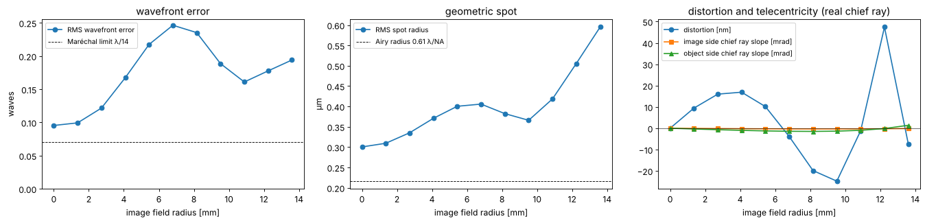
r =  0.00 mm: RMS wavefront 0.095 waves, spot 0.30 µm rms, distortion    +0 nm, chief ray  +0.0 /  +0.0 mrad (object / image)
r =  1.36 mm: RMS wavefront 0.099 waves, spot 0.31 µm rms, distortion    +9 nm, chief ray  -0.4 /  -0.1 mrad (object / image)
r =  2.72 mm: RMS wavefront 0.122 waves, spot 0.34 µm rms, distortion   +16 nm, chief ray  -0.7 /  -0.2 mrad (object / image)
r =  4.08 mm: RMS wavefront 0.167 waves, spot 0.37 µm rms, distortion   +17 nm, chief ray  -1.0 /  -0.2 mrad (object / image)
r =  5.44 mm: RMS wavefront 0.218 waves, spot 0.40 µm rms, distortion   +10 nm, chief ray  -1.3 /  -0.3 mrad (object / image)
r =  6.80 mm: RMS wavefront 0.246 waves, spot 0.41 µm rms, distortion    -4 nm, chief ray  -1.4 /  -0.3 mrad (object / image)
r =  8.16 mm: RMS wavefront 0.235 waves, spot 0.38 µm rms, distortion   -20 nm, chief ray  -1.5 /  -0.3 mrad (object / image)
r =  9.52 mm: RMS wavefront 0.189 waves, spot 0.37 µm rms, distortion   -25 nm, chief ray  -1.4 /  -0.3 mrad (object / image)
r = 10.88 mm: RMS wavefront 0.161 waves, spot 0.42 µm rms, distortion    -1 nm, chief ray  -1.0 /  -0.3 mrad (object / image)
r = 12.24 mm: RMS wavefront 0.178 waves, spot 0.51 µm rms, distortion   +47 nm, chief ray  -0.2 /  -0.3 mrad (object / image)
r = 13.60 mm: RMS wavefront 0.194 waves, spot 0.60 µm rms, distortion    -7 nm, chief ray  +1.4 /  -0.2 mrad (object / image)

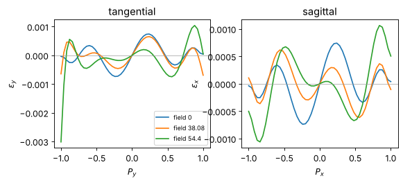
axes = design.plot_ray_fan(fields=[0.0, 0.7*h, h])

The wavefront in Zernike polynomials

System.zernike() fits Fringe Zernike polynomials (peak value 1 on the rim of the pupil) to the OPD map against the reference sphere around the chief ray image point. Z1 (piston) carries no information; Z2/Z3 (tilt) is the shift of the diffraction focus against the chief ray, Z4 a defocus, the rest the aberrations proper. In the field centre only rotationally symmetric terms remain (Z4, Z9, Z16, Z25: defocus and spherical aberration of 4th, 6th and 8th order); at the edge of the field (a y field, mirror symmetric in x) the terms even in x join them: cos mφ for even m (astigmatism, tetrafoil) and sin mφ for odd m (y tilt, y coma, trefoil).

from pyoptics.bases import fringe_to_n_m

J = np.arange(2, 26)
names = {2: "tilt x", 3: "tilt y", 4: "defocus", 5: "astig 0°", 6: "astig 45°", 7: "coma x",
         8: "coma y", 9: "spherical", 10: "trefoil", 11: "trefoil", 12: "astig 2", 13: "astig 2",
         14: "coma 2", 15: "coma 2", 16: "spherical 2", 17: "tetrafoil", 18: "tetrafoil",
         19: "trefoil 2", 20: "trefoil 2", 21: "astig 3", 22: "astig 3", 23: "coma 3", 24: "coma 3",
         25: "spherical 3"}
# RMS of each (peak normalized) Fringe Zernike over the unit disk
rms_norm = np.array([np.sqrt((1 + (fringe_to_n_m(j)[1] == 0))/(2*(fringe_to_n_m(j)[0] + 1))) for j in J])
zfields = [(0.0, "field centre"), (1.0, "field edge (r = 13.6 mm)")]
coeffs = [design.zernike(f*h, 25, N=64)[1:] for f, _ in zfields]

fig, ax = plt.subplots(figsize=(16, 4.5))
for k, ((f, label), c) in enumerate(zip(zfields, coeffs)):
    ax.bar(J + 0.4*(k - 0.5), 1e3*c, width=0.4, label=label)
ax.axhline(0, color="k", lw=0.5)
ax.set_xticks(J)
ax.set_xticklabels([f"Z{j}\n{names[j]}" for j in J], fontsize=8)
ax.set_ylabel("Fringe Zernike coefficient [mλ]")
ax.set_title("wavefront of the corrected lens, Z2 to Z25 (λ = 248.3 nm)")
ax.legend()
fig.tight_layout()

for (f, label), c in zip(zfields, coeffs):
    largest = np.argsort(-np.abs(c*rms_norm))[:4]
    print(f"{label}: RMS of Z2-Z25 {np.sqrt(np.sum((c*rms_norm)**2)):.3f} waves, of the whole OPD "
          f"{np.std(design._valid_opd(f*h, 64, False)):.3f} waves; largest (RMS) "
          + ", ".join(f"Z{J[i]} {1e3*c[i]*rms_norm[i]:+.0f} mλ" for i in largest))

field centre: RMS of Z2-Z25 0.094 waves, of the whole OPD 0.095 waves; largest (RMS) Z16 +66 mλ, Z25 -57 mλ, Z9 -25 mλ, Z4 +25 mλ

field edge (r = 13.6 mm): RMS of Z2-Z25 0.225 waves, of the whole OPD 0.227 waves; largest (RMS) Z3 -116 mλ, Z9 +99 mλ, Z5 -89 mλ, Z17 +75 mλ

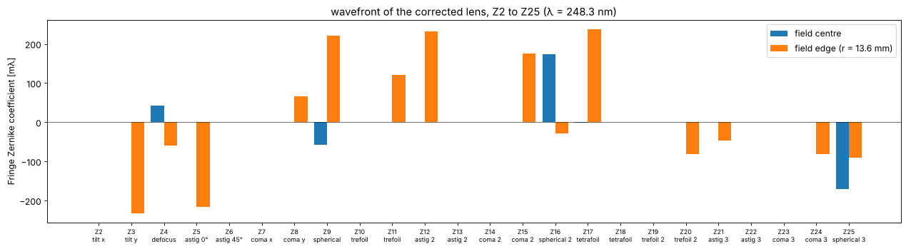
Z2–Z25 hold practically all of the wavefront error at both fields. In the field centre what is left is high order spherical aberration, Z16 and Z25 (6th and 8th order) balanced against each other and against Z9 and defocus; the aspheres (up to \(r^8\)) and the spheres cannot remove the higher orders that NA 0.7 brings. At the field edge the largest term is the tilt Z3: a coefficient \(c\) (peak, in waves) shifts the diffraction focus by \(c\,\lambda/\mathrm{NA}\) against the chief ray, here about 80 nm, so a printed feature sees a “distortion” that differs from that of the chief ray in section 6 by that much; an optimization for overlay would control the centroid, not the chief ray. Next come astigmatism of 2nd and 3rd order (Z5, Z12), spherical aberration (Z9) and tetrafoil (Z17): field dependent aberrations of high order.

7. What the diagram did and what it did not

• First order is exact. The layout of section 3 fixes magnification, NA, length, telecentricity and the flat Petzval field before a single surface is bent; thickening keeps all of it, and the optimizer only has to hold it (the solves for length and NA, small residuals for telecentricity and magnification).

• The correction moves the layout. The diagram of the corrected lens (section 6) keeps the telecentric ends, the strong last bulge around the stop and both waists, but it lowers the bulge between them to almost the height of the waists (marginal ray heights of 50–65 instead of 30–90 in the units of the plot) and pulls the first waist closer to the reticle: the optimizer spread the negative power of the waists over a long, slim middle section.

• 20 elements and 5 aspheres get close to the diffraction limit. The design is corrected to 0.10–0.25 waves RMS over the field (0.3–0.6 µm spots), 1.4–3.5 times the Maréchal limit, with distortions below 50 nm and a real chief ray that leaves the reticle at less than 1.5 mrad and meets the wafer at less than 0.3 mrad: telecentric on both sides. The 13 spherical elements of an earlier version of this notebook reached only 0.5–1.3 waves and gave up the object side telecentricity (170 mrad) for it. Both the extra lenses and the aspheres count: the same 20 elements without aspheres stopped at 0.3–0.6 waves (and 50–60 mrad off telecentric).

• Telecentricity of which ray? Without ray aiming the “chief ray” of the optimizer starts towards the paraxial entrance pupil; at NA 0.7 the pupil aberrations put it tens of mrad away from the ray through the centre of the stop, so a design that was telecentric for the optimizer was not telecentric at all. The aim=True operands of phase 3 trace the real chief ray (aimed at the stop centre by Newton’s method, all fields in one trace), at about twice the cost of an evaluation.

• Not a production design. Real KrF lenses of this NA have about 30 elements; the last element here is a 108 mm thick block in front of the wafer, many air spaces sit at the 1 mm limit and many lenses at the 10 mm limit, and nothing was toleranced. Distortion and wavefront error are only controlled at the sampled fields (the distortion peaks at 47 nm between the 85 % and the full field).

Exercises: sample more fields for distortion; give the optimizer more aspheres or other surfaces for them (aspheres= of LensOptimizer); split the block in front of the wafer (draw another lens into the sketch); use a smaller field or a lower NA and see how the residual wavefront error drops; follow the diagram through the stages of the optimization (DelanoDiagram.from_system()).

print(f"run time {time.time() - t_start:.0f} s")

run time 57 s

References

• E. Delano, “First-order design and the y, ybar diagram”, Appl. Opt. 2, 1251-1256 (1963).

• R. V. Shack, “Analytic system design with pencil and ruler”, Proc. SPIE 39, 127 (1973).

• F. J. López-López, The application of the Delano y-ybar diagram to optical design, Ph.D. dissertation, University of Arizona (1973).

• R. Kingslake and R. B. Johnson, Lens Design Fundamentals, 2nd ed., Academic Press (2010).

• T. Matsuyama, Y. Ohmura and D. M. Williamson, “The lithographic lens: its history and evolution”, Proc. SPIE 6154, 615403 (2006).