Polarization ray tracing with coatings

raytrace.System.trace_polarization() follows the polarization and the power of every ray through a system: each surface multiplies the field with Chipman’s \(3\times3\) polarization ray tracing matrix

\[P = t_s\,\hat s\hat s^T + t_p\,\hat p'\hat p^T,\]

whose Fresnel coefficients come from the bare interface or from the thin film stack (coatings.Coating) on the surface, evaluated at the local angle of incidence of the ray. Mirrors reflect through their coating on a substrate, and the media between the surfaces can absorb (materials.Isotropic, \(n + ik\)) or be birefringent and dichroic (materials.Uniaxial, materials.CubicCrystal).

This notebook coats the ArF water immersion lens of Zeiss patent US 7,187,503 B2 (raytrace.zeiss_arfi_lens(): 193.368 nm, NA 1.35, all fused silica in helium, 43 surfaces) with realistic DUV antireflection coatings and looks at:

1. the angles of incidence in the lens and the design of a two layer AR coating from fluoride materials,

2. the energy budget of the lens (reflection and absorption losses through the pupil and surface by surface),

3. the polarization the coatings leave in the Jones pupil (diattenuation, retardance),

4. layer thickness variations across strongly curved surfaces,

5. the decomposition into apodization, coating phase and a Jones pupil in orientation Zernikes, on axis and through the field, for the lithography projector,

6. a protected aluminium fold mirror.

import numpy as np
import matplotlib.pyplot as plt
from scipy.optimize import minimize

from pyoptics.coatings import Coating, Layer, RadialProfile
from pyoptics.litho import jones_pupil as jp
from pyoptics.litho.plot import plot_orientation
from pyoptics.raytrace import CoordinateBreak, Rays, Surface, System, SIO2_ARF, WATER_ARF, zeiss_arfi_lens

plt.rcParams.update({"figure.dpi": 100, "font.size": 11})

1. Coating materials at 193 nm

Few coating materials are transparent enough for ArF. Production DUV AR coatings are built from fluorides, typically MgF\(_2\) as the low index material and LaF\(_3\) (or GdF\(_3\)) as the high index material; oxides like Al\(_2\)O\(_3\) are used as well, while HfO\(_2\) and TiO\(_2\) absorb too much. Typical indices of evaporated films at 193 nm are (order of magnitude for the extinction, which depends strongly on the deposition process and is larger than at 248 nm):

material	\(n\)	\(k\)
MgF\(_2\)	1.43	\(\sim 5\cdot10^{-4}\)
LaF\(_3\)	1.70	\(\sim 10^{-3}\)
fused silica (substrate)	1.561	\(\approx 0\)

The extinction coefficients make the coatings absorb up to \(10^{-3}\) of the light at every surface, which adds up over 42 coated surfaces and is part of the energy budget below. Indices are given as complex numbers \(n + ik\) with \(k > 0\) (the pyoptics convention \(\exp(i(\mathbf k\cdot\mathbf r - \omega t))\)).

system = zeiss_arfi_lens()
wl = system.wavelength  # mm
n_glass = SIO2_ARF
MgF2, LaF3 = 1.43 + 5e-4j, 1.70 + 1e-3j
print("wavelength {:.1f} nm, fused silica n = {:.4f}, water n = {:.4f}".format(
    system.wavelength_nm, n_glass, WATER_ARF))

wavelength 193.4 nm, fused silica n = 1.5608, water n = 1.4366

Angles of incidence in the lens

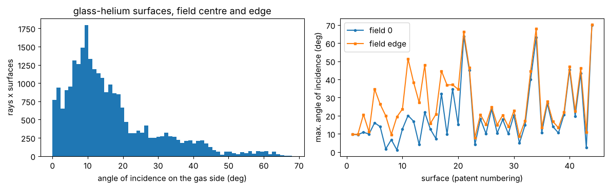
The coating has to work over the angles of incidence that occur in the lens. We trace a grid of pupil rays at the centre and at the edge of the field and collect the angle between ray and local surface normal at every surface, converted to the gas side of the surface (Snell’s law), which is the angle a coating design uses:

def angles_of_incidence(system, field, N=21):
    p = np.linspace(-1, 1, N)
    PX, PY = np.meshgrid(p, p)
    inside = PX**2 + PY**2 <= 1
    bundle = system.trace_pupil(field, PX[inside], PY[inside])
    frames = system.frames()[0]
    n = system.n
    aoi = []
    for i, s in enumerate(system.surfaces):
        o, R = frames[i]
        ok = bundle.valid
        Q = (bundle.points[i + 1][ok] - o) @ R
        cos_i = np.abs(np.sum(s.normal(Q)*(bundle.directions[i][ok] @ R), axis=-1))
        # n sin(i) is conserved; on a glass-gas surface this is the angle on the gas side
        sin_gas = n[i]*np.sqrt(1 - np.clip(cos_i, 0, 1)**2)/min(n[i], n[i + 1])
        aoi.append(np.degrees(np.arcsin(np.clip(sin_gas, 0, 1))))
    return aoi

n_s = len(system.surfaces)
aoi = angles_of_incidence(system, 0.0) + angles_of_incidence(system, system.max_field)
gas = [i for i in range(n_s) if system.n[i] != system.n[i + 1] and min(system.n[i], system.n[i + 1]) < 1.1]
aoi_all = np.concatenate([aoi[i] for i in gas] + [aoi[n_s + i] for i in gas])
fig, axes = plt.subplots(1, 2, figsize=(12, 3.8))
axes[0].hist(aoi_all, bins=60, color="C0")
axes[0].set_xlabel("angle of incidence on the gas side (deg)"), axes[0].set_ylabel("rays x surfaces")
axes[0].set_title("glass-helium surfaces, field centre and edge")
labels = [int(s.label) for s in system.surfaces]
axes[1].plot(labels, [a.max() for a in aoi[:n_s]], "o-", ms=3, label="field 0")
axes[1].plot(labels, [a.max() for a in aoi[n_s:]], "s-", ms=3, label="field edge")
axes[1].set_xlabel("surface (patent numbering)"), axes[1].set_ylabel("max. angle of incidence (deg)")
axes[1].legend()
plt.tight_layout()
print("median {:.1f} deg, 90th percentile {:.1f} deg, 99th percentile {:.1f} deg, max {:.1f} deg".format(
    *np.percentile(aoi_all, [50, 90, 99, 100])))

median 12.7 deg, 90th percentile 35.2 deg, 99th percentile 59.0 deg, max 68.0 deg

Single layer versus two layer AR coating

A quarter wave of MgF\(_2\) (as in the Jones pupil notebook) would need \(n = \sqrt{1.561} = 1.25\) for zero reflection; with the real \(n = 1.43\) it leaves about 2 % per surface. A two layer coating (gas | MgF\(_2\) | LaF\(_3\) | glass) works with real materials and comes close to zero over a range of angles. We optimize the two thicknesses for the smallest mean reflectance (s and p averaged) between 0° and 45°, which holds most rays of the lens; the steep surfaces near the wafer see more, and production coatings are designed surface by surface for their own angle range.

angles = np.radians(np.linspace(0, 45, 46))
print("rays within the design range: {:.0%}".format(np.mean(aoi_all <= 45)))

def mean_R(coating):
    p = coating.power(angles, 1.0, n_glass, wl)
    return np.mean((p["R_s"] + p["R_p"])/2)

def two_layer(d_MgF2, d_LaF3):  # thicknesses in nm, layers from the air side
    return Coating([Layer(MgF2, d_MgF2*1e-6, label="MgF2"), Layer(LaF3, d_LaF3*1e-6, label="LaF3")])

single = Coating([Layer.quarter_wave(MgF2, wl, label="MgF2")])
best = min((minimize(lambda d: mean_R(two_layer(*d)), d0, method="Nelder-Mead")
            for d0 in [(34, 28), (34, 57), (45, 22)]), key=lambda r: r.fun)
d_MgF2, d_LaF3 = best.x
vcoat = two_layer(d_MgF2, d_LaF3)
print("single layer: MgF2 {:.1f} nm, mean R = {:.2%}".format(single.layers[0].thickness*1e6,
                                                            mean_R(single)))
print("two layer:    MgF2 {:.1f} nm, LaF3 {:.1f} nm, mean R = {:.3%}".format(d_MgF2, d_LaF3,
                                                                          mean_R(vcoat)))

rays within the design range: 96%
single layer: MgF2 33.8 nm, mean R = 1.97%
two layer:    MgF2 35.4 nm, LaF3 29.4 nm, mean R = 0.400%

theta = np.radians(np.linspace(0, 70, 141))
fig, axes = plt.subplots(1, 2, figsize=(12, 4))
bare = Coating()
for c, name, ls in ((bare, "uncoated", ":"), (single, "MgF$_2$ $\\lambda/4$", "--"),
                    (vcoat, "MgF$_2$/LaF$_3$", "-")):
    p = c.power(theta, 1.0, n_glass, wl)
    for pol, color in (("s", "C0"), ("p", "C3")):
        axes[0].plot(np.degrees(theta), 100*p["R_" + pol], ls=ls, color=color,
                     label="{} {}".format(name, pol))
    axes[1].plot(np.degrees(theta), 100*(p["A_s"] + p["A_p"])/2, ls=ls, color="k", label=name)
axes[0].set_ylim(0, 10), axes[0].set_ylabel("reflectance (%)")
axes[1].set_ylabel("absorptance (%), unpolarized")
for ax in axes:
    ax.axvspan(0, 45, color="0.9", zorder=0)
    ax.set_xlabel("angle of incidence in air (deg)")
    ax.legend(fontsize=8)
plt.tight_layout()

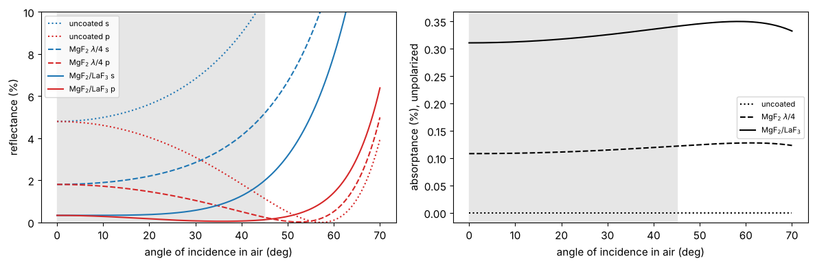
The two layer coating keeps the reflectance around half a percent and below up to about 45° (grey), at the price of a small absorption in the LaF\(_3\) layer. Beyond the design range the reflectance rises quickly, and s and p separate: this is where the coating creates diattenuation.

2. Coating the lens

The coating is attached to every glass–helium surface; the last surface, glass to water, reflects only 0.3 % and stays bare. The layers of a Coating are listed in the order the light meets them, so on the exit surfaces of the lens elements (glass → helium) the stack is reversed().

def coat(system, coating, profile=None):
    # a copy of the system with the coating on every glass-gas surface
    coated = system.copy()
    n = coated.n
    for i, s in enumerate(coated.surfaces):
        if n[i] == n[i + 1] or min(n[i], n[i + 1]) > 1.1:  # no change, or glass to water
            continue
        c = coating if profile is None else profile(s, coating)
        s.coating = c if n[i] < n[i + 1] else c.reversed()
    return coated

variants = {"uncoated": system, "MgF2 single layer": coat(system, single),
            "MgF2/LaF3": coat(system, vcoat)}

p = np.linspace(-1, 1, 41)
PX, PY = np.meshgrid(p, p)
inside = PX**2 + PY**2 <= 1
traced = {name: s.trace_pupil_polarization(0.0, PX[inside], PY[inside])
          for name, s in variants.items()}
for name, t in traced.items():
    T = t.transmittance()
    print("{:18s} transmittance: centre {:.3f}, mean {:.3f}, min {:.3f}".format(
        name, T[np.argmin(PX[inside]**2 + PY[inside]**2)], np.nanmean(T), np.nanmin(T)))

uncoated           transmittance: centre 0.133, mean 0.131, min 0.124
MgF2 single layer  transmittance: centre 0.452, mean 0.431, min 0.385
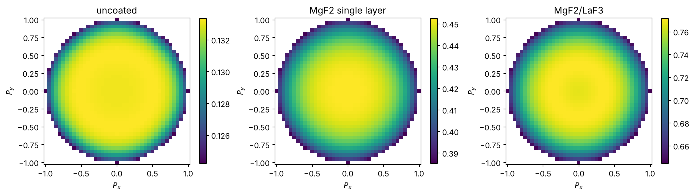
MgF2/LaF3          transmittance: centre 0.766, mean 0.733, min 0.644

Transmission over the pupil

The transmittance of the rays is the apodization of the lens, here for unpolarized light. With 43 surfaces the uncoated lens transmits only 13 %, the single layer 43 % and the two layer coating 73 % (pupil means). The transmission is highest in the centre of the pupil and falls by about 15 % (relative) towards the rim (note the colour scales), where the rays meet the steep surfaces near the wafer beyond the design range of the coating. For unpolarized light the losses of s and p change in opposite directions with the angle of incidence and partly cancel; the difference between s and p shows up in the Jones pupil (section 3).

fig, axes = plt.subplots(1, 3, figsize=(14, 4))
for ax, (name, t) in zip(axes, traced.items()):
    T = np.full(PX.shape, np.nan)
    T[inside] = t.transmittance()
    im = ax.pcolormesh(p, p, T, shading="auto", cmap="viridis")
    ax.set_aspect("equal"), ax.set_title(name)
    ax.set_xlabel("$P_x$"), ax.set_ylabel("$P_y$")
    plt.colorbar(im, ax=ax, shrink=0.85)
plt.tight_layout()

Energy budget surface by surface

PolarizedBundle.power() gives the power that is left behind every surface. For the chief ray and a marginal ray of the coated lens, the steps are the reflection and absorption losses of the individual surfaces. Comparing with the lossless coating (the same layers with \(k = 0\)) separates the two:

lossless = two_layer(d_MgF2, d_LaF3)
for layer in lossless.layers:
    layer.material = layer.material.real
rays = (0.0, [0.0, 0.0], [0.0, 1.0])  # chief and marginal ray at field 0
power = {name: s.trace_pupil_polarization(*rays).power()
         for name, s in (("MgF2/LaF3", variants["MgF2/LaF3"]),
                         ("MgF2/LaF3, k = 0", coat(system, lossless)))}

fig, ax = plt.subplots(figsize=(8, 4))
planes = np.arange(power["MgF2/LaF3"].shape[0])
for (name, P), ls in zip(power.items(), ("-", "--")):
    ax.step(planes, P[:, 0], where="post", ls=ls, color="C0", label=name + ", chief ray")
    ax.step(planes, P[:, 1], where="post", ls=ls, color="C3", label=name + ", marginal ray")
ax.set_xlabel("plane (0: object, 1...{0}: behind the surfaces, {1}: image)".format(n_s, n_s + 1))
ax.set_ylabel("power")
ax.legend(fontsize=8)
plt.tight_layout()
T, T0 = power["MgF2/LaF3"][-1], power["MgF2/LaF3, k = 0"][-1]
print("chief ray: transmitted {:.3f}, reflected {:.3f}, absorbed {:.3f}".format(T[0], 1 - T0[0],
                                                                            T0[0] - T[0]))
print("marginal ray: transmitted {:.3f}, reflected {:.3f}, absorbed {:.3f}".format(T[1], 1 - T0[1],
                                                                               T0[1] - T[1]))

chief ray: transmitted 0.766, reflected 0.127, absorbed 0.106
marginal ray: transmitted 0.644, reflected 0.264, absorbed 0.092

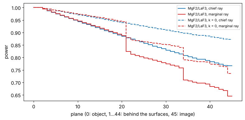
(The split is approximate: the lossless stack also reflects slightly differently.) With these extinction coefficients the absorption of the coatings is of the same order as their residual reflection, which is why coating absorption (and its heating of the lens, lens heating) matters in DUV lithography.

3. Polarization: the Jones pupil

PolarizedBundle.jones() returns the Jones matrices between the aplanatic bases of the object and image space rays; jones_pupil.decompose() splits them into transmission, scalar phase, linear diattenuation and linear retardance (orientators: magnitude and axis). The maps use the entrance pupil coordinates of the rays:

fig, axes = plt.subplots(2, 3, figsize=(14, 8.4))
for col, (name, t) in enumerate(traced.items()):
    ok = t.valid
    parts = jp.decompose(t.jones()[ok])
    d, g = parts["diattenuation"], parts["retardance"]
    xy = (PX[inside][ok], PY[inside][ok])
    plot_orientation(xy + (d[0] + 1j*d[1],), ax=axes[0, col], title=name + "\ndiattenuation")
    plot_orientation(xy + (g[0] + 1j*g[1],), ax=axes[1, col], title="retardance (waves)")
plt.tight_layout()

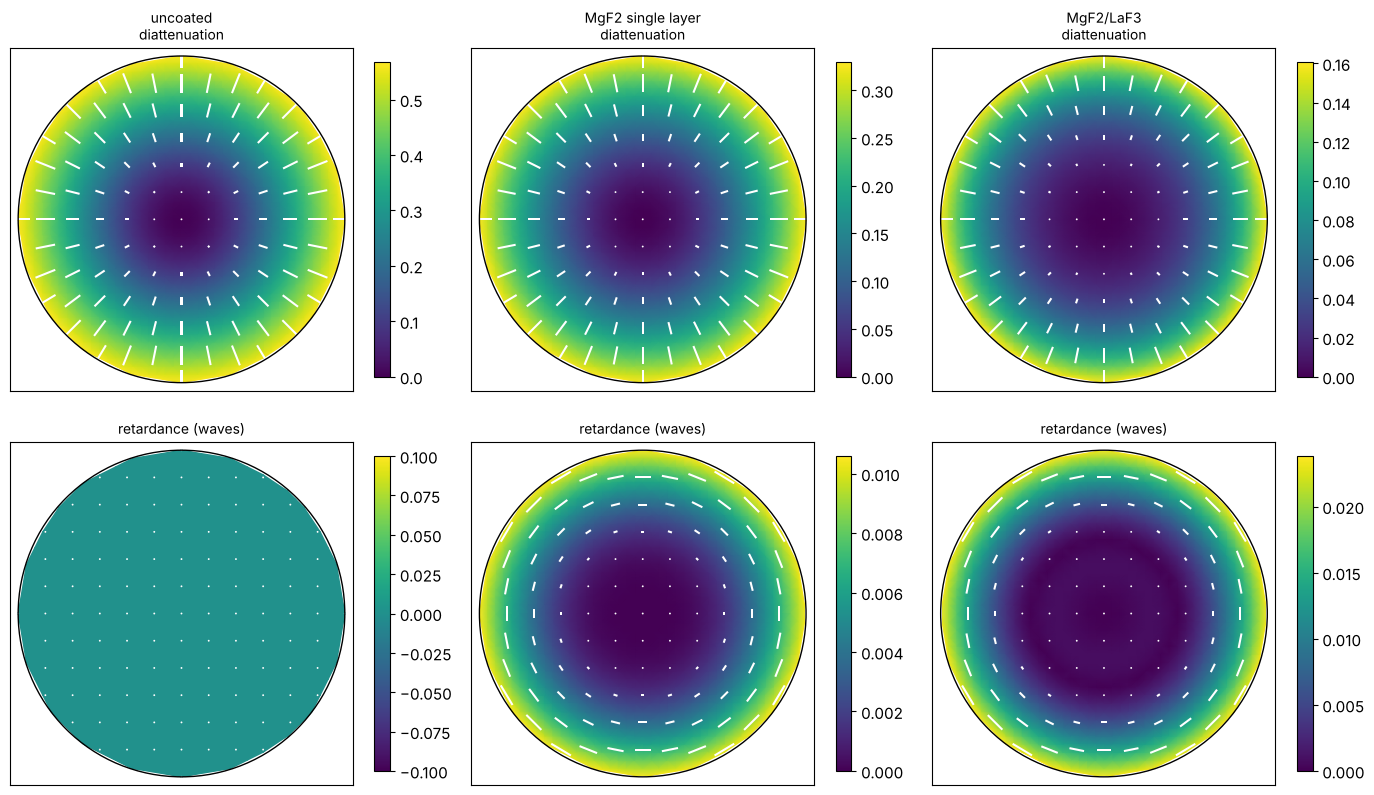
The uncoated lens is a radial diattenuator with no retardance (real Fresnel coefficients). Both coatings reduce the diattenuation strongly, but add retardance that grows towards the rim of the pupil, since the phases of \(t_s\) and \(t_p\) of a thin film stack separate with the angle of incidence. The two layer coating has the smaller diattenuation and a retardance of about a hundredth of a wave.

4. Layer thickness variations on curved surfaces

In an evaporation plant the layers grow thinner towards the rim of a strongly curved lens, roughly with the cosine of the local slope angle of the surface, \(t(r) \approx t_0 \cos\alpha(r)\) with \(\sin\alpha = r/R\) for a sphere. To second order this is \(t/t_0 \approx 1 - \tfrac12 (r/R)^2\), a RadialProfile with \(a_2 = -\tfrac12 (r_\mathrm{max}/R)^2\) on \(\rho = r/r_\mathrm{max}\). The profile is evaluated at the hit point of every ray in the local surface coordinates.

def cosine_falloff(surface, coating):
    r_max = surface.semi_diameter
    a2 = -0.5*(r_max/surface.R)**2 if np.isfinite(surface.R) else 0.0
    return Coating([Layer(l.material, l.thickness, RadialProfile([a2], r_norm=r_max), l.label)
                    for l in coating.layers])

profiled = coat(system, vcoat, profile=cosine_falloff)
rim = sorted(((-0.5*(s.semi_diameter/s.R)**2, s.label) for s in system.surfaces))[:5]
print("strongest thinning at the rim:",
      ", ".join("surface {}: {:.0%}".format(i, a) for a, i in rim))

t_prof = profiled.trace_pupil_polarization(0.0, PX[inside], PY[inside])
fig, axes = plt.subplots(1, 3, figsize=(14, 4.2))
results = {}
for name, t in (("uniform", traced["MgF2/LaF3"]), ("cosine falloff", t_prof)):
    ok = t.valid
    parts = jp.decompose(t.jones()[ok])
    results[name] = t, ok, parts
    g = parts["retardance"]
    rho = np.hypot(PX[inside][ok], PY[inside][ok])
    axes[0].plot(rho, np.hypot(*g[:2]), ".", ms=2, label=name)
    axes[1].plot(rho, t.transmittance()[ok], ".", ms=2, label=name)
axes[0].set_ylabel("|retardance| (waves)"), axes[1].set_ylabel("transmittance")
for ax in axes[:2]:
    ax.set_xlabel("pupil radius"), ax.legend(markerscale=5)
t, ok, parts = results["cosine falloff"]
g = parts["retardance"]
plot_orientation((PX[inside][ok], PY[inside][ok], g[0] + 1j*g[1]), ax=axes[2],
                 title="retardance (waves), cosine falloff")
plt.tight_layout()

strongest thinning at the rim: surface 43: -42%, surface 14: -38%, surface 41: -35%, surface 17: -33%, surface 34: -32%

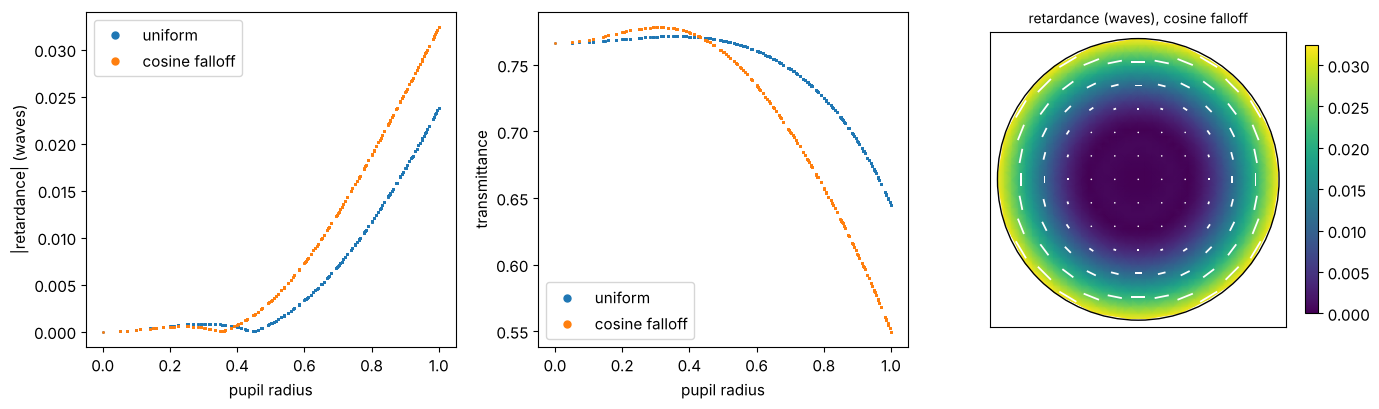
Thinner layers shift the reflectance minimum of the coating to shorter wavelengths, which at a fixed wavelength acts like a larger angle of incidence: the transmission at the rim of the pupil drops and the retardance changes. Uniformity masks in the coating plant are used to keep such profiles within specification; with RadialProfile, PolynomialProfile or ZernikeProfile (or any function of the local \(x, y\)) measured or modelled profiles go straight into the ray trace.

5. Decomposition: Jones pupil and apodization

For imaging, the lithography projector (litho.Projector) describes the lens by a scalar pupil (apodization, i.e. the amplitude transmission, and the wavefront in Zernikes) plus a Jones pupil that holds only the polarization and leaves the mean transmission and phase alone. The polar decomposition \(J = \sqrt{T}\,e^{i\Phi}\,U H\) (jones_pupil.decompose()) separates the two:

• the mean intensity transmission \(T\) gives the apodization \(A = \sqrt{T}\) relative to the chief ray, fitted as Fringe Zernikes \(A = 1 + \sum_j a_j Z_j\) (the linear apodization model of Projector),

• the scalar phase \(\Phi\) is the coating phase, a wavefront error on top of the geometric OPD of the lens (in waves, Zernikes),

• the retarder \(U\) and the diattenuator \(H\) form the Jones pupil, fitted with orientation Zernikes (PhysicalJonesPupil.fit()).

litho.lens.lens_jones_pupil() traces the lens with the coatings attached to its surfaces, on the normalized pupil coordinates of the projector, and normalizes \(J\) to the chief ray. All four variants, including the coating with the cosine falloff:

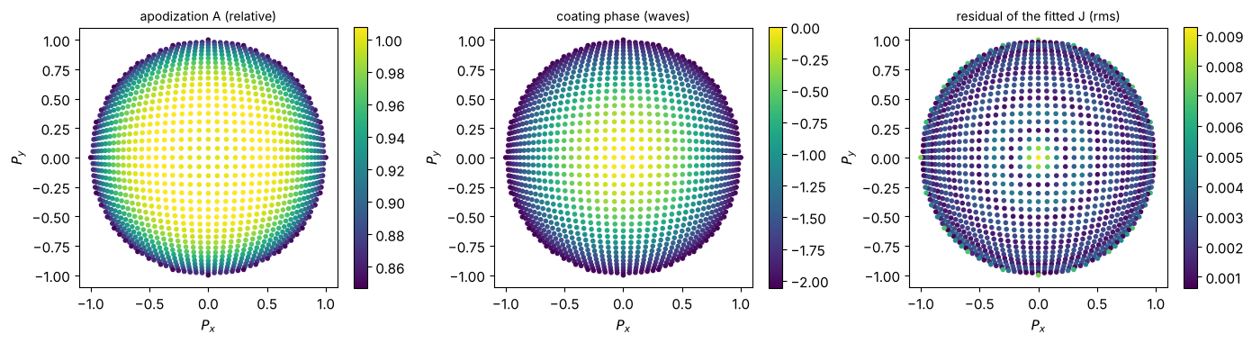
The coating phase of all 42 coated surfaces adds up to more than half a wave at the rim of the pupil for the coating with the thickness falloff, so the phase from decompose() (taken modulo \(2\pi\)) is unwrapped first (pyoptics.unwrap, on the grid of entrance pupil rays that lens_jones_pupil() traces).

from pyoptics.litho import lens
from pyoptics.unwrap import unwrap

N_pupil, n_terms = 41, 25
_, PXg, PYg, inside_g = System._pupil_grid(N_pupil)

def unwrapped(phase):
    # the rays of lens_jones_pupil() are the entrance pupil grid points
    assert len(phase) == inside_g.sum(), "vignetted rays: map them to the grid first"
    grid = np.zeros(PXg.shape)
    grid[inside_g] = phase
    u = unwrap(grid, mask=inside_g)[inside_g]
    return u - u[np.argmin(PXg[inside_g]**2 + PYg[inside_g]**2)]

all_variants = dict(variants)
all_variants["MgF2/LaF3, cosine falloff"] = profiled
pupils, fits = {}, {}
for name, s in all_variants.items():
    r = lens.lens_jones_pupil(s, N=N_pupil)
    parts = jp.decompose(r.J)
    parts["phase"] = unwrapped(parts["phase"])
    physical, _ = jp.PhysicalJonesPupil.fit(r.P_x, r.P_y, r.J, n_terms=n_terms)
    coating_phase = jp.fit_zernikes(r.P_x, r.P_y, parts["phase"]/(2*np.pi), n_terms)
    apodization = jp.fit_zernikes(r.P_x, r.P_y, np.sqrt(parts["transmission"]) - 1, n_terms)
    pupils[name], fits[name] = (r, parts), (physical, coating_phase, apodization)

def show(coefficients, keys, fmt="{:+.4f}"):
    return "  ".join("{}: {}".format(k, fmt.format(coefficients.get(k, 0.0))) for k in keys)

for name, (physical, coating_phase, apodization) in fits.items():
    print("{} (chief ray transmission {:.3f})".format(name, pupils[name][0].transmission))
    print("  diattenuation OZ  ", show(physical.diattenuation, (5, 12, 21)))
    print("  retardance OZ     ", show(physical.retardance, (5, 12, 21)))
    print("  apodization Z     ", show(apodization, (4, 9, 16)))
    print("  coating phase Z   ", show(coating_phase, (4, 9, 16)), "(waves)")

uncoated (chief ray transmission 0.133)
  diattenuation OZ   5: +0.4977  12: +0.0557  21: +0.0118
  retardance OZ      5: +0.0000  12: +0.0000  21: +0.0000
  apodization Z      4: -0.0079  9: -0.0094  16: -0.0068
  coating phase Z    4: +0.0000  9: +0.0000  16: +0.0000 (waves)
MgF2 single layer (chief ray transmission 0.452)
  diattenuation OZ   5: +0.2615  12: +0.0484  21: +0.0154
  retardance OZ      5: -0.0068  12: -0.0030  21: -0.0007
  apodization Z      4: -0.0271  9: -0.0188  16: -0.0090
  coating phase Z    4: -0.1949  9: -0.0110  16: -0.0042 (waves)
MgF2/LaF3 (chief ray transmission 0.766)
  diattenuation OZ   5: +0.1036  12: +0.0366  21: +0.0161
  retardance OZ      5: -0.0123  12: -0.0091  21: -0.0019
  apodization Z      4: -0.0285  9: -0.0247  16: -0.0102
  coating phase Z    4: -0.3494  9: -0.0190  16: -0.0075 (waves)
MgF2/LaF3, cosine falloff (chief ray transmission 0.766)
  diattenuation OZ   5: +0.1489  12: +0.0676  21: +0.0261
  retardance OZ      5: -0.0200  12: -0.0110  21: -0.0011
  apodization Z      4: -0.0667  9: -0.0426  16: -0.0075
  coating phase Z    4: -1.0122  9: -0.0401  16: -0.0156 (waves)

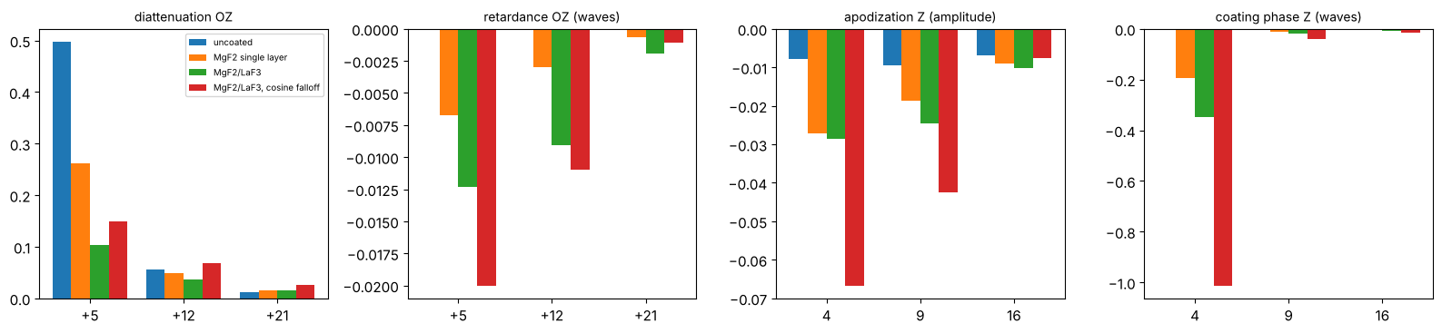
The centred lens only has the rotationally symmetric terms: OZ \(+5, +12, +21\) for radial (positive) or tangential (negative) diattenuation and retardance, \(Z_4, Z_9, Z_{16}\) for apodization and coating phase. Side by side:

groups = (("diattenuation OZ", lambda f: f[0].diattenuation, (5, 12, 21)),
          ("retardance OZ (waves)", lambda f: f[0].retardance, (5, 12, 21)),
          ("apodization Z (amplitude)", lambda f: f[2], (4, 9, 16)),
          ("coating phase Z (waves)", lambda f: f[1], (4, 9, 16)))
fig, axes = plt.subplots(1, 4, figsize=(16, 3.8))
width = 0.8/len(fits)
for ax, (title, get, keys) in zip(axes, groups):
    for k, (name, f) in enumerate(fits.items()):
        c = get(f)
        ax.bar(np.arange(len(keys)) + (k - (len(fits) - 1)/2)*width, [c.get(j, 0.0) for j in keys],
               width, label=name)
    ax.set_xticks(range(len(keys)))
    ax.set_xticklabels(["{:+d}".format(j) if "OZ" in title else str(j) for j in keys])
    ax.axhline(0, color="0.5", lw=0.6)
    ax.set_title(title, fontsize=10)
axes[0].legend(fontsize=7)
plt.tight_layout()

The apodization itself, \(A = \sqrt{T/T_\mathrm{chief}}\) over the pupil radius (points: traced rays, lines: the Zernike fit along \(P_y = 0\)):

fig, ax = plt.subplots(figsize=(7, 4))
rho_line = np.linspace(0, 1, 101)
for k, (name, ((r, parts), (physical, coating_phase, apodization))) in enumerate(
        zip(fits, zip(pupils.values(), fits.values()))):
    ax.plot(np.hypot(r.P_x, r.P_y), np.sqrt(parts["transmission"]), ".", ms=2, color="C{}".format(k),
            alpha=0.4)
    ax.plot(rho_line, 1 + jp.zernike_sum(apodization, rho_line, 0*rho_line).real,
            color="C{}".format(k), label=name)
ax.set_xlabel("pupil radius"), ax.set_ylabel("apodization A")
ax.legend(fontsize=8)
plt.tight_layout()

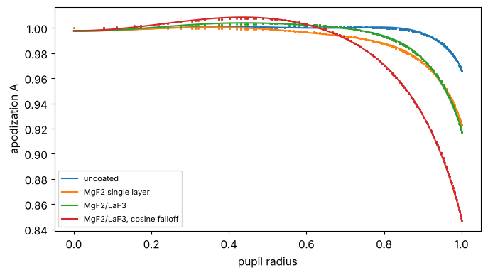
The uncoated lens is dominated by radial diattenuation (OZ \(+5 \approx 0.5\)); its apodization for unpolarized light is weak, as the losses of s and p compensate. The coatings reduce the diattenuation by a factor of two (single layer) to five (0.10 for the two layer coating) and bring in a tangential retardance (negative OZ \(+5\), \(+12\) of up to about a hundredth of a wave) and a coating phase: \(-0.35\) waves of \(Z_4\) for the two layer coating, a defocus that the lens design (or the focus of the scanner) compensates, and a little spherical aberration (\(Z_9\)). The thickness falloff increases diattenuation and retardance, adds an apodization that falls off towards the rim (\(Z_4\), \(Z_9\) of the amplitude) and triples the defocus-like coating phase.

Apodization and coating phase maps, and the quality of the fits

The maps of the decomposition and the residual of the fitted pupil, \(\sqrt{T}e^{i\Phi}\,U H\) rebuilt from 25 Zernikes and OZPs each, for the coating with the thickness falloff:

name = "MgF2/LaF3, cosine falloff"
(r, parts), (physical, coating_phase, apodization) = pupils[name], fits[name]
A = 1 + jp.zernike_sum(apodization, r.P_x, r.P_y).real
phase = 2*np.pi*jp.zernike_sum(coating_phase, r.P_x, r.P_y).real
J_fit = (A*np.exp(1j*phase))[:, None, None]*physical(r.P_x, r.P_y)
residual = np.linalg.norm(J_fit - r.J, axis=(1, 2))/np.sqrt(2)

fig, axes = plt.subplots(1, 3, figsize=(14, 4))
for ax, v, title in ((axes[0], np.sqrt(parts["transmission"]), "apodization A (relative)"),
                     (axes[1], parts["phase"]/(2*np.pi), "coating phase (waves)"),
                     (axes[2], residual, "residual of the fitted J (rms)")):
    sc = ax.scatter(r.P_x, r.P_y, c=v, s=9, cmap="viridis")
    ax.set_aspect("equal"), ax.set_title(title, fontsize=10)
    ax.set_xlabel("$P_x$"), ax.set_ylabel("$P_y$")
    plt.colorbar(sc, ax=ax, shrink=0.85)
plt.tight_layout()
print("max residual of the fitted Jones pupil: {:.1e}".format(residual.max()))

max residual of the fitted Jones pupil: 9.3e-03

Through the field

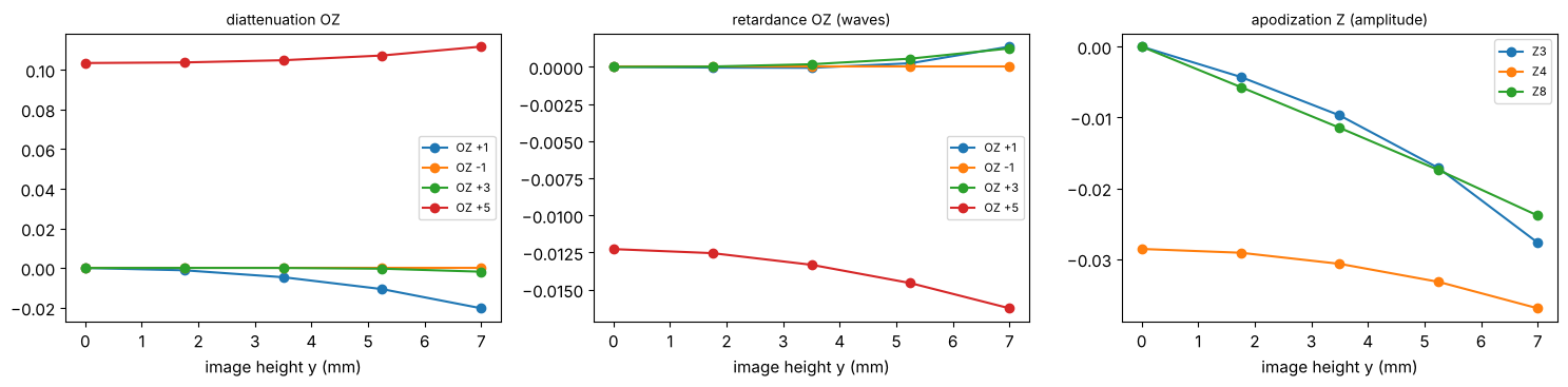
Off axis the symmetry is broken: the chief ray crosses the surfaces obliquely, and constant and tilt-like terms (OZ \(\pm1\), \(\pm2\), \(\pm3\); \(Z_2, Z_3\) in the apodization) appear, growing with the field like distortion and coma in the wavefront. Field points are image heights in mm along y:

coated = variants["MgF2/LaF3"]
heights = np.linspace(0, 7.0, 5)
rows = []
for h in heights:
    r = lens.lens_jones_pupil(coated, field=(0.0, h), N=31)
    physical, scalar = jp.PhysicalJonesPupil.fit(r.P_x, r.P_y, r.J, n_terms=16)
    apodization = jp.fit_zernikes(r.P_x, r.P_y, np.sqrt(jp.decompose(r.J)["transmission"]) - 1, 16)
    rows.append((physical.diattenuation, physical.retardance, apodization))
fig, axes = plt.subplots(1, 3, figsize=(15, 3.8))
for ax, (k, keys, title) in zip(axes, ((0, (1, -1, 3, 5), "diattenuation OZ"),
                                       (1, (1, -1, 3, 5), "retardance OZ (waves)"),
                                       (2, (3, 4, 8), "apodization Z (amplitude)"))):
    for j in keys:
        ax.plot(heights, [row[k].get(j, 0.0) for row in rows], "o-",
                label=("OZ {:+d}" if "OZ" in title else "Z{}").format(j))
    ax.set_xlabel("image height y (mm)"), ax.set_title(title, fontsize=10)
    ax.legend(fontsize=8)
plt.tight_layout()

Hand-off to the lithography projector

The pieces go straight into Projector: the geometric wavefront from projector_from_system() plus the coating phase as Zernikes, the apodization Zernikes and the fitted PhysicalJonesPupil (see notebooks 33 and 38 for imaging with them):

name = "MgF2/LaF3"
physical, coating_phase, apodization = fits[name]
projector = lens.projector_from_system(all_variants[name], n_terms=n_terms, n=WATER_ARF,
                                       apodization_zernikes=apodization,
                                       jones_pupil=physical)
wavefront = dict(projector.zernikes)
for j, c in coating_phase.items():
    if j > 1:  # piston does not matter
        wavefront[j] = wavefront.get(j, 0.0) + c
projector = projector.with_(zernikes=wavefront)
print("NA {:.3f}, wavelength {:.1f} nm".format(projector.NA, projector.wavelength))
print("coating phase Z4, Z9 (waves): {:+.4f}, {:+.4f}".format(coating_phase[4], coating_phase[9]))
print("lens + coating Z4, Z9 (waves): {:+.4f}, {:+.4f}".format(wavefront.get(4, 0.0),
                                                              wavefront.get(9, 0.0)))

NA 1.348, wavelength 193.4 nm
coating phase Z4, Z9 (waves): -0.3494, -0.0190
lens + coating Z4, Z9 (waves): -0.3447, -0.0581

6. A protected aluminium fold mirror

Folded lens designs (catadioptric lithography lenses) use fold mirrors at large angles of incidence. Bare aluminium oxidizes, so it is protected by a dielectric overcoat, here MgF\(_2\). Aluminium at 193 nm has \(n \approx 0.11 + 2.2i\) (Rakić, Appl. Opt. 34, 4755 (1995)). The coating of a mirror lists its layers from the incidence side and names the substrate:

Al = 0.11 + 2.2j
d = np.linspace(0, 120, 241)  # MgF2 overcoat thickness in nm
R_s, R_p, delta = [], [], []
for di in d:
    c = Coating([Layer(MgF2, di*1e-6)], substrate=Al)
    p = c.power(np.pi/4, 1.0, wavelength=wl)
    r_s, r_p = c.amplitudes(np.cos(np.pi/4), 1.0, None, wl)[:2]
    R_s.append(p["R_s"]), R_p.append(p["R_p"])
    delta.append(np.angle(-r_p/r_s))  # phase of p relative to s (full field)
fig, axes = plt.subplots(1, 2, figsize=(12, 4))
axes[0].plot(d, 100*np.array(R_s), label="$R_s$")
axes[0].plot(d, 100*np.array(R_p), label="$R_p$")
axes[0].set_ylabel("reflectance at 45° (%)")
axes[1].plot(d, np.degrees(np.unwrap(delta)))
axes[1].set_ylabel("phase p - s at 45° (deg)")
for ax in axes:
    ax.set_xlabel("MgF$_2$ overcoat (nm)")
axes[0].legend()
plt.tight_layout()

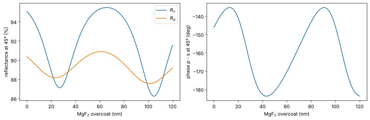
The overcoat changes reflectance and retardance of the mirror periodically with its optical thickness. In a system, the mirror is a Surface(mirror=True, coating=...). Here a collimated beam is folded by 90° about the x axis with coordinate breaks; the Jones matrix of the chief ray is diagonal in s (\(x\)) and p, with the retardance and diattenuation of the coating:

protected = Coating([Layer(MgF2, 25e-6, label="MgF2")], substrate=Al)
fold = System([Surface(thickness=10.0, semi_diameter=10.0),
               CoordinateBreak(tilt=(np.pi/4, 0, 0)),
               Surface(mirror=True, coating=protected),
               CoordinateBreak(tilt=(np.pi/4, 0, 0), thickness=-10.0)], 0, wl)
t = fold.trace_polarization(Rays([[0.0, 0.0, -1.0]], [[0.0, 0.0, 1.0]], [0.0]))
J = t.jones()[0]
parts = jp.decompose(J)
print("Jones matrix of the fold:\n", np.round(J, 4))
print("power: s {:.4f}, p {:.4f}, unpolarized {:.4f}".format(
    t.transmittance((1, 0))[0], t.transmittance((0, 1))[0], t.transmittance()[0]))
print("diattenuation {:.4f}, retardance {:.4f} waves".format(
    np.hypot(*parts["diattenuation"][:2]), np.hypot(*parts["retardance"][:2])))

Jones matrix of the fold:
 [[0.9076-0.2215j 0.    +0.j    ]
 [0.    +0.j     0.9118+0.2243j]]
power: s 0.8729, p 0.8818, unpolarized 0.8773
diattenuation 0.0051, retardance 0.0765 waves

Summary

• coatings.Layer and coatings.Coating describe thin film stacks with complex indices; Coating.power() checks a design over the angle of incidence.

• Attached to the surfaces of a raytrace.System (Surface(coating=...)), they enter the polarization ray trace at the local angle of incidence of every ray, with thickness profiles across the surface.

• PolarizedBundle gives the power along every ray (reflection and absorption losses, apodization), the output fields and the Jones matrices for litho.jones_pupil.

• litho.lens.lens_jones_pupil() uses the coatings of the surfaces; the polar decomposition separates apodization (amplitude Zernikes) and coating phase (wavefront Zernikes) from the Jones pupil (orientation Zernikes), which together describe the lens in litho.Projector.

• Absorbing and birefringent media (materials.Isotropic, materials.Uniaxial, materials.CubicCrystal) are traced the same way; see the Jones pupil notebook for the intrinsic birefringence of CaF\(_2\).

References

• G. Yun, K. Crabtree and R. A. Chipman, “Three-dimensional polarization ray-tracing calculus I: definition and diattenuation”, Appl. Opt. 50, 2855-2865 (2011).

• G. Yun, S. C. McClain and R. A. Chipman, “Three-dimensional polarization ray-tracing calculus II: retardance”, Appl. Opt. 50, 2866-2874 (2011).

• R. A. Chipman, W.-S. T. Lam and G. Young, Polarized Light and Optical Systems, CRC Press (2018).

• H. A. Macleod, Thin-Film Optical Filters, 3rd ed., Institute of Physics Publishing (2001).

• A. D. Rakić, “Algorithm for the determination of intrinsic optical constants of metal films: application to aluminum”, Appl. Opt. 34, 4755-4767 (1995).

• G. R. McIntyre, J. Kye, H. Levinson and A. R. Neureuther, “Polarization aberrations in hyper-numerical-aperture projection printing: a comparison of various representations”, J. Micro/Nanolith. MEMS MOEMS 5, 033001 (2006).