Interferometry: phase shifting and Fourier fringe analysis

An interferometer superposes a test beam, which carries the wavefront error \(W\) of the optics under test as the phase \(\varphi = kW\), with a reference beam. The camera sees the two-beam interferogram

\[I = |E_\mathrm{test} + E_\mathrm{ref}\,e^{i\delta}|^2 = a + b\cos(\varphi - \delta) = a\,[1 + \gamma\cos(\varphi - \delta)],\]

with the bias \(a\), the fringe amplitude \(b\) and the modulation (visibility) \(\gamma = b/a\). One frame has three unknowns per pixel, so the phase needs either several frames with known phase shifts \(\delta_j\) (phase-shifting interferometry, PSI) or a single frame with a tilt carrier whose spectrum separates the information (Fourier-transform method, Takeda 1982).

pyoptics.interferometry offers:

Function	Frames	Shifts
psi_n_step(frames, shifts)	\(N \ge 3\)	any known shifts (least squares)
psi_4_step(frames)	4	\(0, \pi/2, \pi, 3\pi/2\)
psi_carre(frames)	4	\(\pm\alpha/2, \pm 3\alpha/2\), \(\alpha\) unknown
psi_hariharan(frames)	5	\(0, \pm\pi/2, \pm\pi\), insensitive to linear shift errors
fourier_fringe_analysis(I, x, y)	1	tilt carrier \(k_c\)

All of them return the wrapped phase and the modulation \(\gamma\); the phase is then unwrapped with pyoptics.unwrap. Simulation helpers: zernike_phase(), interferogram(), interfere() and phase_shifts().

Sign convention. pyoptics fields vary as \(e^{i(\mathbf{k}\cdot\mathbf{r} - \omega t)}\), so a wavefront that runs ahead has \(\varphi > 0\) (phase \(= +k\cdot\)OPD). The algorithms return \(\varphi = \arg(E_\mathrm{test}E_\mathrm{ref}^*)\). A phase shift \(\delta > 0\) delays the reference, hence \(\cos(\varphi - \delta)\). Many textbooks write \(\cos(\varphi + \delta)\); their formulas give \(-\varphi\) here. Image stacks have the frame index last, as everywhere in pyoptics.processing.

import warnings

import numpy as np
import matplotlib.pyplot as plt
from scipy.ndimage import binary_erosion

from pyoptics.bases import FringeZernikes
from pyoptics.fft import FT
from pyoptics.interferometry import (zernike_phase, interferogram, interfere,
                                     phase_shifts, psi_n_step, psi_4_step,
                                     psi_carre, psi_hariharan,
                                     shift_error_sensitivity,
                                     fourier_fringe_analysis, find_carrier)
from pyoptics.processing import CameraNoiser
from pyoptics.unwrap import wrap, unwrap_ls
from pyoptics.utils import grid2d, freq_grid

plt.rcParams.update({"figure.dpi": 80, "image.origin": "lower", "font.size": 11})


def show(ax, img, title, cmap="viridis", **kwargs):
    im = ax.imshow(img, extent=extent, cmap=cmap, **kwargs)
    ax.set_title(title)
    ax.set_xticks([]); ax.set_yticks([])
    plt.colorbar(im, ax=ax, fraction=0.046, pad=0.04)
    return im


def nan_outside(img, mask):
    return np.where(mask, img, np.nan)


N = 256
x, y, X, Y = grid2d(-1, 1, -1, 1, N)
extent = (x[0], x[-1], y[0], y[-1])

0. The interferometer

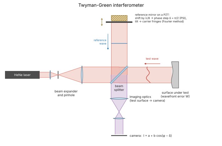
A Twyman-Green interferometer, the setup behind the frames below. The expanded laser beam is split into a reference arm, which ends on a flat mirror, and a test arm, which picks up the wavefront error \(W\) of the optics under test (here a surface in reflection, drawn exaggerated). Both return through the beam splitter, and a telescope images the test surface onto the camera, so that every pixel sees \(I = a + b\cos(\varphi - \delta)\) for one point of the surface. A piezo actuator (PZT) moves the reference mirror: a shift of \(\lambda/8\) lengthens the reference path by \(\lambda/4\), a phase step of \(\delta = \pi/2\) (sections 2 to 4). Tilting the mirror instead adds the linear carrier phase of the Fourier method (section 5). A Fizeau interferometer (notebook 24) does the same with a common path: its reference is a surface in the test beam.

from pyoptics import sketch

fig, ax = plt.subplots(figsize=(11, 6))
sketch.twyman_green(ax, title="Twyman-Green interferometer")
plt.tight_layout()

1. The test wavefront and its interferograms

A wavefront in a pupil of radius 0.9 with 2.5 waves of defocus plus astigmatism, coma and spherical aberration (Fringe Zernike coefficients in waves). Four phase-shifted frames with shifts \(0, \pi/2, \pi, 3\pi/2\): with every step of \(\pi/2\) the fringes move by a quarter period, towards larger \(\varphi\), i.e. outwards for this wavefront that runs ahead at the edge.

coeffs = {4: 2.5, 5: -0.6, 6: 0.3, 7: 0.4, 9: 0.25}       # waves
phi, pupil = zernike_phase(x, y, list(coeffs.values()), 0.9, indices=list(coeffs))
gamma_true = 0.85

shifts = phase_shifts(4)
frames = interferogram(phi, visibility=gamma_true, shift=shifts) * pupil[..., None]

fig, axes = plt.subplots(1, 5, figsize=(19, 3.6))
show(axes[0], nan_outside(phi/(2*np.pi), pupil), "wavefront W (waves)")
for j in range(4):
    show(axes[j + 1], frames[..., j], r"frame %d: $\delta$ = %d°" % (j + 1, np.degrees(shifts[j])),
         cmap="gray")
plt.tight_layout()

interfere() builds the same frames from two complex fields: here the test field \(e^{i\varphi}\) and a weaker reference. The visibility is then \(\gamma = 2|E_t||E_r|/(|E_t|^2 + |E_r|^2)\).

E_ref = 0.5
frames_fields = interfere(np.exp(1j*phi), E_ref, shifts)
rec, gamma = psi_4_step(frames_fields)
print("max phase error: %.1e rad" % np.max(np.abs(wrap(rec - phi))[pupil]))
print("modulation: %.4f (expected %.4f)" % (gamma[pupil].mean(), 2*E_ref/(1 + E_ref**2)))

max phase error: 1.8e-15 rad
modulation: 0.8000 (expected 0.8000)

2. Phase-shifting algorithms

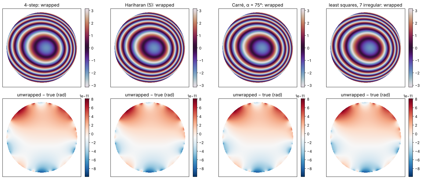
All four algorithms recover the wrapped phase exactly from noise-free frames, each with its own shift sequence. Carré’s algorithm does not even need to know the step: it estimates \(\alpha\) from the frames (here \(\alpha = 75°\)). Least-squares unwrapping inside the pupil gives back the wavefront, and a Zernike fit returns the coefficients.

cases = {
    "4-step": (psi_4_step, phase_shifts(4)),
    "Hariharan (5)": (psi_hariharan, phase_shifts(5, np.pi/2, -np.pi)),
    "Carré, α = 75°": (psi_carre, phase_shifts(4, np.radians(75), -1.5*np.radians(75))),
    "least squares, 7 irregular": (None, np.sort(np.random.default_rng(3).uniform(0, 2*np.pi, 7))),
}

fig, axes = plt.subplots(2, 4, figsize=(18, 7.5))
results = {}
for i, (name, (func, sh)) in enumerate(cases.items()):
    fr = interferogram(phi, visibility=gamma_true, shift=sh)
    if func is None:
        psi, gam = psi_n_step(fr, sh)
    else:
        psi, gam = func(fr)
    u = unwrap_ls(nan_outside(psi, pupil), mask=pupil)
    err = u - phi
    err -= err[pupil].mean()
    results[name] = u
    show(axes[0, i], nan_outside(psi, pupil), name + ": wrapped", cmap="twilight")
    show(axes[1, i], nan_outside(err, pupil), "unwrapped − true (rad)", cmap="RdBu_r")
    print("%-28s max error %.1e rad, modulation %.4f" % (name, np.abs(err[pupil]).max(), gam[pupil].mean()))
plt.tight_layout()

print("Carré's estimated step: %.4f°" % np.degrees(psi_carre(
    interferogram(phi, shift=cases["Carré, α = 75°"][1]), return_step=True)[2]))

4-step                       max error 9.9e-11 rad, modulation 0.8500

Hariharan (5)                max error 9.9e-11 rad, modulation 0.8500

Carré, α = 75°               max error 9.9e-11 rad, modulation 0.8500

least squares, 7 irregular   max error 9.9e-11 rad, modulation 0.8500

Carré's estimated step: 75.0000°

Z = FringeZernikes(x, y, R_norm=0.9)
idx = list(range(1, 10))
fit = Z.coeffs_from_field(np.nan_to_num(results["4-step"])/(2*np.pi), idx)
print(" j   true (waves)   fit (waves)")
for j, c in zip(idx, fit):
    if j > 1:   # piston is arbitrary
        print("%2d   %10.6f   %11.6f" % (j, coeffs.get(j, 0.0), c))

 j   true (waves)   fit (waves)
 2     0.000000      0.000000
 3     0.000000      0.000000
 4     2.500000      2.500000
 5    -0.600000     -0.600000
 6     0.300000      0.300000
 7     0.400000      0.400000
 8     0.000000     -0.000000
 9     0.250000      0.250000

3. Phase shifter miscalibration

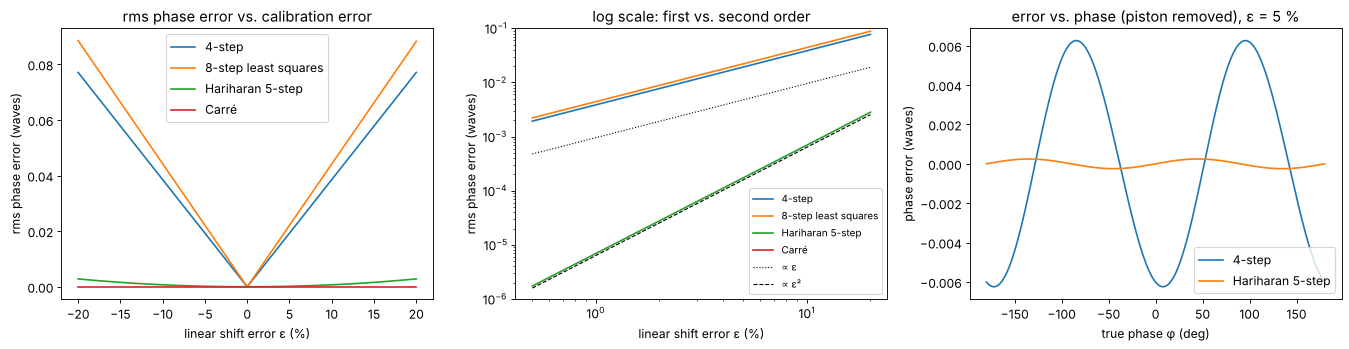
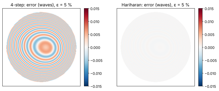
A real phase shifter (a piezo moving the reference mirror) never moves exactly as commanded. With a linear calibration error \(\delta_j' = \delta_j(1 + \varepsilon)\), the four-bucket algorithm produces a phase error that oscillates at twice the fringe frequency (“print-through” of the fringes) with an amplitude proportional to \(\varepsilon\), plus a harmless piston. Hariharan’s five-frame algorithm was designed to cancel the first order, so its error grows only with \(\varepsilon^2\). Carré’s algorithm estimates the actual step and is immune to a linear error, but it is more sensitive to noise (Section 4). shift_error_sensitivity() computes the rms error over all phases.

eps = np.linspace(-0.2, 0.2, 81)
algos = [("4-step", {}), ("n-step", dict(N=8)), ("hariharan", {}), ("carre", {})]
labels = {"4-step": "4-step", "n-step": "8-step least squares", "hariharan": "Hariharan 5-step",
          "carre": "Carré"}

fig, axes = plt.subplots(1, 3, figsize=(17, 4.5))
for name, kw in algos:
    rms = shift_error_sensitivity(name, eps, **kw)
    axes[0].plot(100*eps, rms/(2*np.pi), label=labels[name])
    axes[1].loglog(100*eps[eps > 0], rms[eps > 0]/(2*np.pi), label=labels[name])
for ax in axes[:2]:
    ax.set_xlabel("linear shift error ε (%)"); ax.set_ylabel("rms phase error (waves)")
axes[1].loglog(100*eps[eps > 0], 0.6*eps[eps > 0]/(2*np.pi), "k:", lw=1, label="∝ ε")
axes[1].loglog(100*eps[eps > 0], 0.4*eps[eps > 0]**2/(2*np.pi), "k--", lw=1, label="∝ ε²")
axes[1].set_ylim(1E-6, 1E-1)
axes[0].legend(); axes[1].legend(fontsize=9)
axes[0].set_title("rms phase error vs. calibration error")
axes[1].set_title("log scale: first vs. second order")

# phase error vs. phase for ε = 5 %: the 2φ ripple
p = np.linspace(-np.pi, np.pi, 721)
for name, func, n, centered in [("4-step", psi_4_step, 4, False),
                                ("Hariharan 5-step", psi_hariharan, 5, True)]:
    sh = phase_shifts(n, np.pi/2, -(n - 1)*np.pi/4 if centered else 0.0, linear_error=0.05)
    rec = func(interferogram(p, shift=sh))[0]
    e = wrap(rec - p)
    axes[2].plot(np.degrees(p), (e - e.mean())/(2*np.pi), label=name)
axes[2].set_xlabel("true phase φ (deg)"); axes[2].set_ylabel("phase error (waves)")
axes[2].set_title("error vs. phase (piston removed), ε = 5 %"); axes[2].legend()
plt.tight_layout()

The ripple at twice the fringe frequency is what one sees in a measured wavefront when the phase shifter is off: the fringe pattern prints through. In the wavefront below, the shifter moves 5 % too far.

fig, axes = plt.subplots(1, 2, figsize=(10, 4))
for ax, (name, func, n, centered) in zip(axes, [("4-step", psi_4_step, 4, False),
                                                ("Hariharan", psi_hariharan, 5, True)]):
    sh = phase_shifts(n, np.pi/2, -(n - 1)*np.pi/4 if centered else 0.0, linear_error=0.05)
    psi = func(interferogram(phi, shift=sh))[0]
    err = wrap(psi - phi)
    err -= np.median(err[pupil])   # the shift error also adds a harmless piston
    show(ax, nan_outside(err/(2*np.pi), pupil), name + ": error (waves), ε = 5 %",
         cmap="RdBu_r", vmin=-0.015, vmax=0.015)
plt.tight_layout()

4. Camera noise

With photon shot noise only, the phase noise of an \(N\)-frame algorithm with equally spaced shifts is \(\sigma_\varphi = 1/(\gamma\sqrt{N I_0/2})\), where \(I_0\) is the mean number of photons per pixel and frame. The frames go through a CameraNoiser (Poisson model). Carré’s algorithm divides by small numbers where \(\sin\varphi\) or \(\cos\varphi\) vanish and is several times noisier.

photons = np.logspace(1.5, 5, 9)
algos = {"4-step": (psi_4_step, phase_shifts(4)),
         "Hariharan": (psi_hariharan, phase_shifts(5, np.pi/2, -np.pi)),
         "8-step LS": (lambda f: psi_n_step(f, phase_shifts(8)), phase_shifts(8)),
         "Carré (α = 90°)": (psi_carre, phase_shifts(4, np.pi/2, -3*np.pi/4))}
noiser = CameraNoiser("poisson", rng=1)
fig, ax = plt.subplots(figsize=(7, 4.5))
for name, (func, sh) in algos.items():
    sig = []
    for I0 in photons:
        fr = interferogram(phi, visibility=gamma_true, shift=sh, I0=I0, noiser=noiser)
        sig.append(np.std(wrap(func(fr)[0] - phi)[pupil]))
    ax.loglog(photons, np.array(sig)/(2*np.pi), "o-", label=name)
for n, ls in [(4, ":"), (8, "--")]:
    ax.loglog(photons, 1/(gamma_true*np.sqrt(n*photons/2))/(2*np.pi), "k" + ls, lw=1,
              label=r"$1/(\gamma\sqrt{N I_0/2})$, N = %d" % n)
ax.set_xlabel("mean photons per pixel and frame"); ax.set_ylabel("rms phase noise (waves)")
ax.legend(fontsize=9); ax.grid(True, which="both", alpha=0.3)
plt.tight_layout()

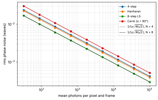
(The Hariharan algorithm weights its five frames unequally, so it sits slightly above the 4-frame limit for its \(N = 5\).)

5. Fourier-transform method (Takeda)

A single frame suffices if the reference is tilted: the carrier \(k_c\) turns the fringes into a nearly periodic pattern \(I = a + c\,e^{i\mathbf{k}_c\cdot\mathbf{r}} + c^*e^{-i\mathbf{k}_c\cdot\mathbf{r}}\) with \(c = \tfrac{b}{2}e^{i\varphi}\). In the spectrum, \(c\) forms a sideband around \(k_c\). A window around \(k_c\) (radius \(|k_c|/2\) by default) isolates it; the inverse transform times \(e^{-i\mathbf{k}_c\cdot\mathbf{r}}\) gives \(c\), hence \(\varphi\) and \(\gamma\). find_carrier() locates the sideband as the centroid of the power spectrum around its peak (give it the pupil mask, otherwise the pupil edge can outshine the sideband).

phi_t, pupil_t = zernike_phase(x, y, [0, 0, 0, 0.8, 0.4, 0, 0.3], 0.9)
kc_true = (2*np.pi*30/2, 2*np.pi*8/2)          # 30 and 8 fringes across the field
I = interferogram(phi_t, x, y, visibility=0.8, carrier=kc_true) * pupil_t
I = CameraNoiser("poisson", rng=4)(500*I)/500        # 500 photons

kc = find_carrier(I, x, y, mask=pupil_t)
print("carrier: found (%.2f, %.2f), true (%.2f, %.2f) rad/unit" % (kc + kc_true))
psi, gam = fourier_fringe_analysis(I, x, y, carrier=kc, mask=pupil_t)
u = unwrap_ls(nan_outside(psi, pupil_t), mask=pupil_t)

# remove piston and tilt (the found carrier may differ slightly from the true one)
A = np.stack([np.ones(pupil_t.sum()), X[pupil_t], Y[pupil_t]], axis=1)
d = (u - phi_t)[pupil_t]
d -= A @ np.linalg.lstsq(A, d, rcond=None)[0]
err = np.full_like(u, np.nan); err[pupil_t] = d

KX, KY = freq_grid(x, y)
S = np.abs(FT(I - I[pupil_t].mean()))
fig, axes = plt.subplots(1, 4, figsize=(19, 4))
show(axes[0], I, "interferogram with carrier", cmap="gray")
im = axes[1].imshow(np.log10(S + S.max()*1E-6), extent=(KX[0, 0], KX[0, -1], KY[0, 0], KY[-1, 0]),
                    cmap="magma")
axes[1].add_patch(plt.Circle(kc, np.hypot(*kc)/2, fill=False, color="c", lw=2))
axes[1].plot(0, 0, "w+"); axes[1].set_xlim(-150, 150); axes[1].set_ylim(-150, 150)
axes[1].set_title("log spectrum and sideband window"); axes[1].set_xlabel("$k_x$"); axes[1].set_ylabel("$k_y$")
show(axes[2], nan_outside(u, pupil_t), "unwrapped phase (rad)")
show(axes[3], err/(2*np.pi), "error after tilt removal (waves)", cmap="RdBu_r", vmin=-0.03, vmax=0.03)
plt.tight_layout()
print("rms error: %.4f waves, inside r < 0.8: %.4f waves" % (np.nanstd(err)/(2*np.pi),
      np.nanstd(np.where(np.hypot(X, Y) < 0.8, err, np.nan))/(2*np.pi)))

carrier: found (95.96, 25.14), true (94.25, 25.13) rad/unit

rms error: 0.0113 waves, inside r < 0.8: 0.0054 waves

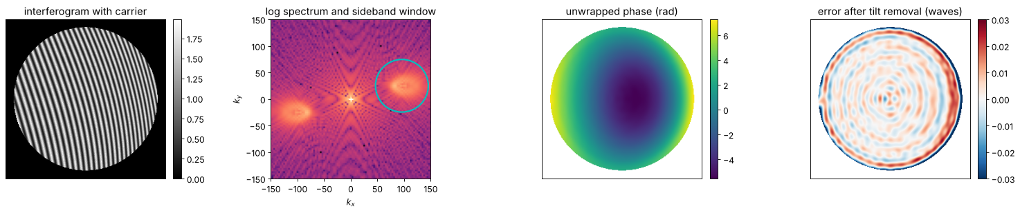
The errors concentrate at the pupil edge: the abrupt end of the fringes spreads the sideband (leakage), and the window cuts off part of it. Inside the pupil, the error is set by the shot noise. The mask argument fills the region outside the pupil with the mean intensity before the transform and sets the outputs there to zero.

Spectral overlap: how large must the carrier be?

The sideband extends over \(k_c \pm \max|\nabla\varphi|\). It must stay clear of the zero order and of the \(-1\) order, otherwise the window catches parts of them. Below, the same wavefront is analysed with ever smaller carriers. The function warns when the window holds less than 90 % of the sideband power. The dashed line marks the carrier at which the steepest local phase gradient equals \(|k_c|/2\).

grad_max = np.max(np.hypot(*np.gradient(phi_t, y, x))[binary_erosion(pupil_t, iterations=2)])
fringes = np.arange(3, 51)
rms, warned = [], []
inner = np.hypot(X, Y) < 0.8
for nf in fringes:
    kc_n = (2*np.pi*nf/2, 0.0)
    I_n = interferogram(phi_t, x, y, visibility=0.8, carrier=kc_n) * pupil_t
    with warnings.catch_warnings(record=True) as w:
        warnings.simplefilter("always")
        p, _ = fourier_fringe_analysis(I_n, x, y, carrier=kc_n, mask=pupil_t)
    warned.append(any("sideband power" in str(wi.message) for wi in w))
    rms.append(np.sqrt(np.mean(wrap(p - phi_t)[inner]**2)))
rms, warned = np.array(rms)/(2*np.pi), np.array(warned)

fig, axes = plt.subplots(1, 3, figsize=(17, 4.2))
axes[0].semilogy(fringes, rms, "-", color="C0")
axes[0].semilogy(fringes[warned], rms[warned], "o", color="C3", label="warning issued")
axes[0].semilogy(fringes[~warned], rms[~warned], "o", color="C0", label="no warning")
axes[0].axvline(2*grad_max/(2*np.pi/2), color="gray", ls="--", label=r"$|k_c|/2 = \max|\nabla\varphi|$")
axes[0].set_xlabel("carrier (fringes across the field)"); axes[0].set_ylabel("rms phase error, r < 0.8 (waves)")
axes[0].legend(fontsize=9)
for ax, nf in zip(axes[1:], [8, 36]):
    kc_n = (2*np.pi*nf/2, 0.0)
    I_n = interferogram(phi_t, x, y, visibility=0.8, carrier=kc_n) * pupil_t
    S_n = np.abs(FT(I_n - I_n[pupil_t].mean()))
    ax.imshow(np.log10(S_n + S_n.max()*1E-5), extent=(KX[0, 0], KX[0, -1], KY[0, 0], KY[-1, 0]), cmap="magma")
    ax.add_patch(plt.Circle(kc_n, np.hypot(*kc_n)/2, fill=False, color="c", lw=2))
    ax.set_xlim(-250, 250); ax.set_ylim(-250, 250)
    ax.set_title("%d fringes: log spectrum" % nf); ax.set_xlabel("$k_x$"); ax.set_ylabel("$k_y$")
plt.tight_layout()

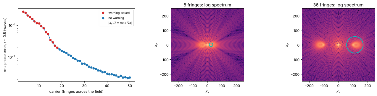
Window shape and apodization

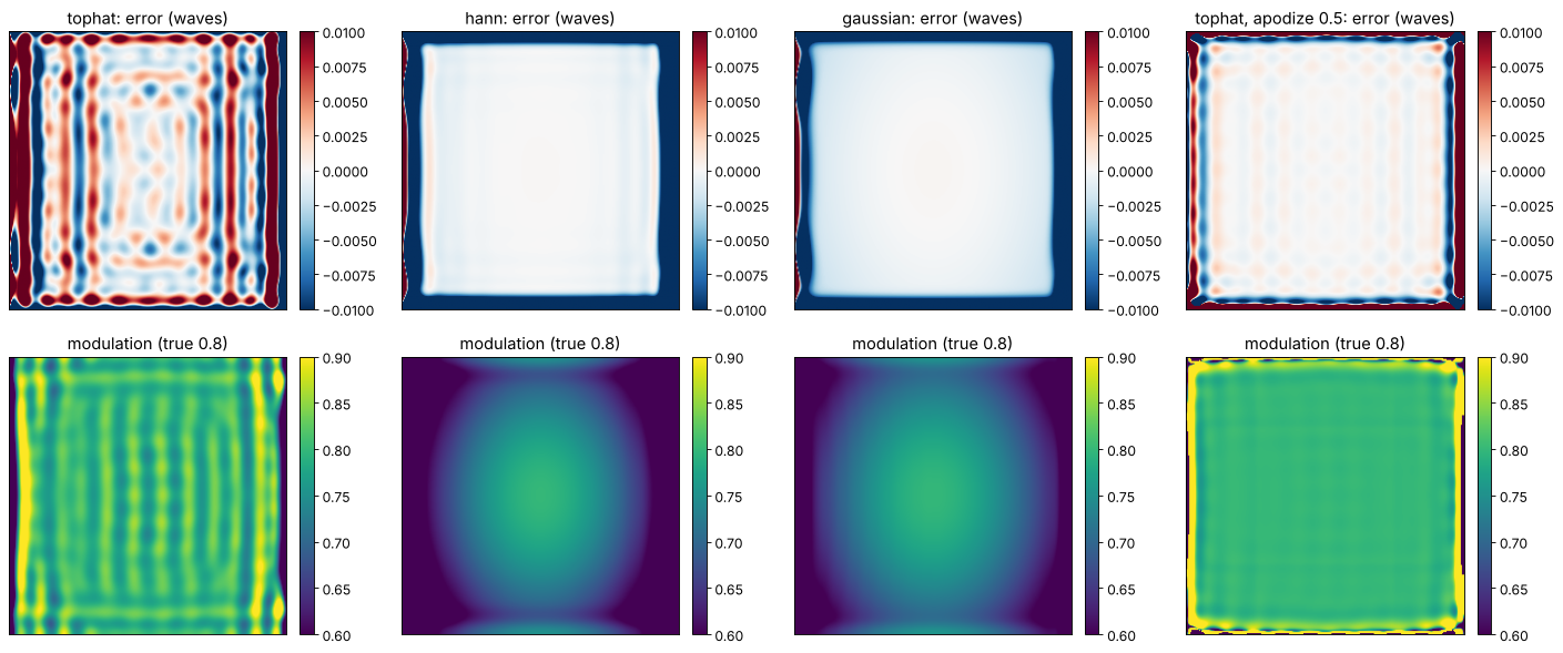
The default top-hat window keeps the sideband unattenuated, so the modulation comes out right. Tapered windows ("hann", "gaussian") ring less but attenuate the outer parts of a broad sideband, which biases \(\gamma\) low where the fringes are dense. Apodizing the frame with a Tukey window (apodize) reduces the ringing that the edges of a full-field interferogram cause in the interior, at the expense of the tapered border. Here the fringes fill the whole frame (no pupil), which is the worst case for leakage.

phi_f, _ = zernike_phase(x, y, [0, 0, 0, 1.0, 0.3], 1.5)
kc_f = (2*np.pi*20.4/2, 0.0)   # non-integer number of fringes: not periodic
I_f = interferogram(phi_f, x, y, visibility=0.8, carrier=kc_f)
cases = [("tophat", 0.0), ("hann", 0.0), ("gaussian", 0.0), ("tophat", 0.5)]
fig, axes = plt.subplots(2, 4, figsize=(18, 7.5))
for i, (win, ap) in enumerate(cases):
    p, g = fourier_fringe_analysis(I_f, x, y, carrier=kc_f, window=win, apodize=ap)
    e = wrap(p - phi_f)
    e -= np.median(e[np.hypot(X, Y) < 0.5])   # piston
    title = "%s%s" % (win, ", apodize %.1f" % ap if ap else "")
    show(axes[0, i], e/(2*np.pi), title + ": error (waves)", cmap="RdBu_r", vmin=-0.01, vmax=0.01)
    show(axes[1, i], g, "modulation (true 0.8)", vmin=0.6, vmax=0.9)
    c = np.hypot(X, Y) < 0.5
    print("%-22s rms error r < 0.5: %.2e waves, median modulation %.3f" %
          (title, np.std(e[c])/(2*np.pi), np.median(g[c])))
plt.tight_layout()

tophat                 rms error r < 0.5: 2.69e-03 waves, median modulation 0.799

hann                   rms error r < 0.5: 9.99e-05 waves, median modulation 0.771
gaussian               rms error r < 0.5: 1.51e-04 waves, median modulation 0.776
tophat, apodize 0.5    rms error r < 0.5: 2.65e-04 waves, median modulation 0.800

Summary

• Use phase shifting whenever the setup allows several frames: the phase is exact without noise, pixel by pixel, without any spatial filtering. Prefer algorithms that tolerate the dominant error: Hariharan’s five frames for shifter calibration errors, more frames against noise (the phase noise falls with \(1/\sqrt{N I_0}\)), Carré if the step is unknown and the light level is high.

• The Fourier-transform method needs a single frame (vibration-insensitive, dynamic measurements) but a carrier large enough to separate the orders, \(|k_c|/2 > \max|\nabla\varphi|\), and it smooths the phase and loses accuracy at the edges.

• Both give the wrapped phase; unwrap it with pyoptics.unwrap, then fit Zernikes with pyoptics.bases.

References

• D. Malacara (ed.), Optical Shop Testing, 3rd ed., Wiley (2007).

• J. H. Bruning, D. R. Herriott, J. E. Gallagher, D. P. Rosenfeld, A. D. White and D. J. Brangaccio, “Digital wavefront measuring interferometer for testing optical surfaces and lenses”, Appl. Opt. 13, 2693-2703 (1974).

• J. E. Greivenkamp, “Generalized data reduction for heterodyne interferometry”, Opt. Eng. 23, 350-352 (1984).

• P. Carré, “Installation et utilisation du comparateur photoélectrique et interférentiel du Bureau International des Poids et Mesures”, Metrologia 2, 13-23 (1966).

• P. Hariharan, B. F. Oreb and T. Eiju, “Digital phase-shifting interferometry: a simple error-compensating phase calculation algorithm”, Appl. Opt. 26, 2504-2506 (1987).

• K. Creath, “Phase-measurement interferometry techniques”, Prog. Opt. 26, 349-393 (1988).

• M. Takeda, H. Ina and S. Kobayashi, “Fourier-transform method of fringe-pattern analysis for computer-based topography and interferometry”, J. Opt. Soc. Am. 72, 156-160 (1982).