Phase retrieval with the transport-of-intensity equation (TIE)
Cameras measure only intensities. A transparent object (e.g. a cell or a glass structure), however, changes almost only the phase and is practically invisible in focus. Defocus a little, and it becomes visible: phase gradients redirect light, curved phase gathers or spreads it like a lens. The transport-of-intensity equation describes this quantitatively:
Two slightly defocused images give \(\partial I/\partial z\), and the equation (a
Poisson equation) can be solved for the phase \(\varphi\). pyoptics.TIE provides
tie() (forward direction), solve_tie() (solution via FFT) and
enhanced_tie_solve() (iterative refinement).
Convention: \(\exp(i(kz - \omega t))\), the field is \(\sqrt{I}\,e^{i\varphi}\). A converging wave (phase falling off outwards, as behind a converging lens) has \(\partial I/\partial z > 0\) on the axis.
import numpy as np
import matplotlib.pyplot as plt

from pyoptics import TIE
from pyoptics.propagators import rayleigh_sommerfeld_I_TF
from pyoptics.utils import grid2d, get_z_derivative

plt.rcParams.update({"figure.dpi": 100, "image.origin": "lower", "font.size": 11})

wl = 0.5
k = 2*np.pi/wl
1. A phase object
Two Gaussian phase bumps (one positive, one negative) in a wide Gaussian beam.
The intensity in focus contains no trace of the object. The defocused images
are computed with propagators.rayleigh_sommerfeld_I_TF() (angular spectrum
method), which uses the same convention.
L, N = 60.0, 256
x, y, X, Y = grid2d(-L/2, L/2, -L/2, L/2, N)
phase = 1.0*np.exp(-((X - 5)**2 + (Y - 3)**2)/(2*1.5**2)) - 0.7*np.exp(-((X + 8)**2 + (Y + 6)**2)/(2*1.0**2))
I0 = np.exp(-(X**2 + Y**2)/(2*20**2))
U0 = np.sqrt(I0)*np.exp(1j*phase)

def intensity_at(z):
    """Intensity after propagation by z. For z < 0 via time reversal (see notebook 15),
    so that rounding errors in evanescent frequencies do not blow up."""
    if z >= 0:
        return np.abs(rayleigh_sommerfeld_I_TF(U0, x, y, z, wl)[0])**2
    return np.abs(rayleigh_sommerfeld_I_TF(np.conj(U0), x, y, -z, wl)[0])**2

ext = (x[0], x[-1], y[0], y[-1])
fig, axes = plt.subplots(1, 4, figsize=(15, 3.6))
im = axes[0].imshow(phase, extent=ext, cmap="RdBu_r", vmin=-1, vmax=1)
fig.colorbar(im, ax=axes[0], fraction=0.046); axes[0].set_title("phase φ [rad]")
for ax, z in zip(axes[1:], (-10, 0, 10)):
    I = intensity_at(z)
    im = ax.imshow(I/I0, extent=ext, cmap="gray", vmin=0.6, vmax=1.4)
    ax.set_title(f"$I(z)/I_0$, $z$ = {z:+d} µm")
fig.colorbar(im, ax=axes[3], fraction=0.046)
for ax in axes:
    ax.set_xlim(-20, 20); ax.set_ylim(-20, 20); ax.set_xlabel("$x$ [µm]")
fig.suptitle("A pure phase object only becomes visible with defocus (with opposite contrast before and behind focus)")
fig.tight_layout()
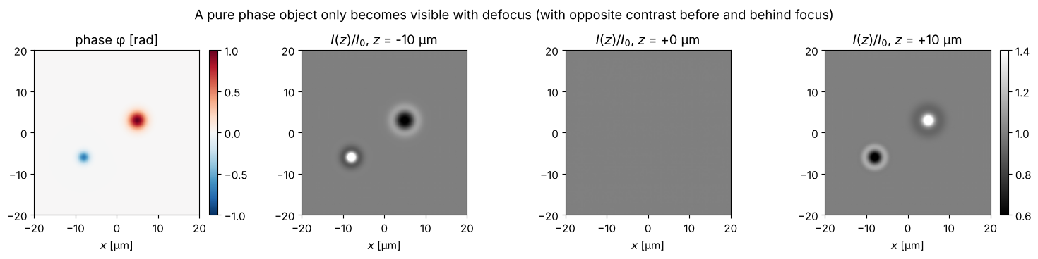
The positive phase bump acts like a converging lens (bright for \(z > 0\)), the negative one like a diverging lens (dark). Before the focus it is the other way round.
2. Forward direction: does the TIE hold?
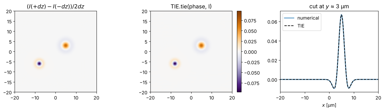
TIE.tie(phase, I, x, y, lam) computes \(\partial I/\partial z\) from the phase. For
comparison, the central difference quotient from two propagated images.
dz = 1.0
dIdz_num = (intensity_at(dz) - intensity_at(-dz))/(2*dz)
dIdz_tie = TIE.tie(phase, I0, x, y, wl)
vmax = np.abs(dIdz_tie).max()
fig, axes = plt.subplots(1, 3, figsize=(13, 3.8))
for ax, D, title in zip(axes[:2], (dIdz_num, dIdz_tie), ("$(I(+dz) - I(-dz))/2dz$", "TIE.tie(phase, I)")):
    im = ax.imshow(D, extent=ext, cmap="PuOr_r", vmin=-vmax, vmax=vmax)
    ax.set_xlim(-20, 20); ax.set_ylim(-20, 20); ax.set_title(title)
fig.colorbar(im, ax=axes[1], fraction=0.046)
axes[2].plot(x, dIdz_num[N//2 + int(3/(x[1]-x[0]))], lw=2.5, alpha=0.6, label="numerical")
axes[2].plot(x, dIdz_tie[N//2 + int(3/(x[1]-x[0]))], "k--", label="TIE")
axes[2].set_xlim(-20, 20); axes[2].set_xlabel("$x$ [µm]"); axes[2].legend(); axes[2].set_title("cut at $y$ ≈ 3 µm")
fig.tight_layout()
3. Backward direction: phase from two images
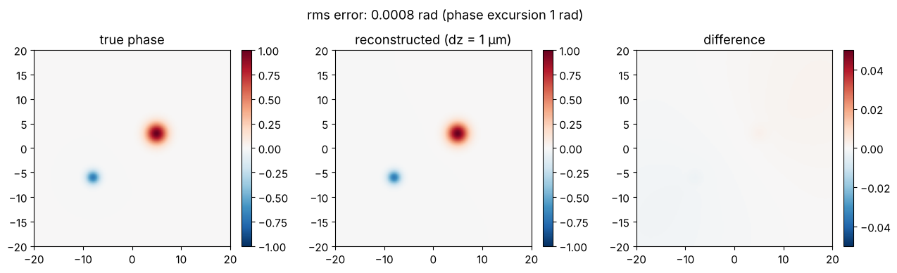
solve_tie(I, dI_dz, x, y, lam, alpha) solves the TIE with two inverse Laplace
operators in Fourier space. The phase is only determined up to a constant; for the
comparison we subtract the mean in the illuminated region.
mask = I0 > 0.2
def rms_error(ph):
    e = (ph - phase)[mask]
    return np.sqrt(np.mean((e - e.mean())**2))

phase_rec = TIE.solve_tie(I0, dIdz_num, x, y, wl, 0.0)
offset = np.mean((phase_rec - phase)[mask])

fig, axes = plt.subplots(1, 3, figsize=(13, 3.8))
for ax, P, title in zip(axes, (phase, phase_rec - offset, phase_rec - offset - phase),
                        ("true phase", "reconstructed (dz = 1 µm)", "difference")):
    lim = 1 if title != "difference" else 0.05
    im = ax.imshow(np.where(mask, P, np.nan), extent=ext, cmap="RdBu_r", vmin=-lim, vmax=lim)
    fig.colorbar(im, ax=ax, fraction=0.046)
    ax.set_xlim(-20, 20); ax.set_ylim(-20, 20); ax.set_title(title)
fig.suptitle(f"rms error: {rms_error(phase_rec):.4f} rad (phase excursion 1 rad)")
fig.tight_layout()
4. The trade-off in the defocus distance
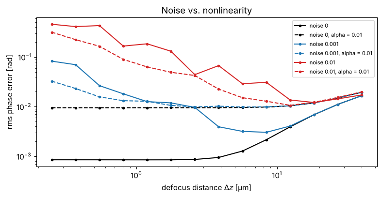
In practice the images are noisy. The difference quotient \((I_+ - I_-)/2\Delta z\) amplifies the noise by \(1/\Delta z\): small distances are sensitive to noise. Large distances, on the other hand, violate the assumption that \(I\) changes linearly with \(z\) (diffraction “smears out” the fine structures). In between lies an optimum that depends on the noise level.
The second parameter is the regularization alpha: the inverse Laplace
operator \(-1/(k_x^2 + k_y^2)\) amplifies low frequencies and thus low-frequency
noise. With alpha > 0 it is damped to \(-1/(k_x^2 + k_y^2 + \alpha)\).
rng = np.random.default_rng(0)
dz_vals = np.logspace(np.log10(0.25), np.log10(40), 14)
noise_levels = (0.0, 1e-3, 1e-2)
fig, ax = plt.subplots(figsize=(8, 4.2))
for noise, c in zip(noise_levels, ("k", "C0", "C3")):
    for alpha, ls in ((0.0, "-"), (1e-2, "--")):
        errs = []
        for dz in dz_vals:
            Ip = intensity_at(dz) + noise*rng.standard_normal(X.shape)
            Im = intensity_at(-dz) + noise*rng.standard_normal(X.shape)
            errs.append(rms_error(TIE.solve_tie(I0, (Ip - Im)/(2*dz), x, y, wl, alpha)))
        label = f"noise {noise:g}" + (f", alpha = {alpha:g}" if alpha else "")
        ax.loglog(dz_vals, errs, ls, color=c, marker="o", ms=3, label=label)
ax.set_xlabel("defocus distance $\\Delta z$ [µm]"); ax.set_ylabel("rms phase error [rad]")
ax.set_title("Noise vs. nonlinearity"); ax.legend(fontsize=8)
fig.tight_layout()
5. More planes: Savitzky-Golay derivative
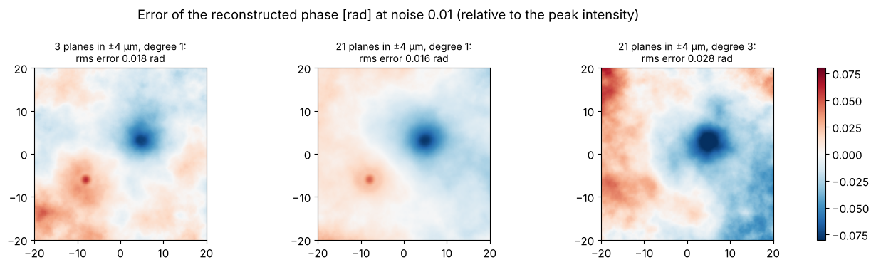
With more than two images, the derivative can be estimated more robustly.
utils.get_z_derivative(stack, dz, order) fits a polynomial to the intensity along
\(z\) in every pixel (Savitzky-Golay) and evaluates its derivative in the central
plane. More planes in the same \(z\) range average out the noise. A higher
polynomial degree would reduce the systematic error due to the nonlinearity, but
amplifies the noise again; in this noise-dominated case, the straight line
(degree 1) is best.
noise = 1e-2
z_max = 4.0
fig, axes = plt.subplots(1, 3, figsize=(13, 3.8))
results = {}
for n_planes, order in ((3, 1), (21, 1), (21, 3)):
    z_planes = np.linspace(-z_max, z_max, n_planes)
    stack = np.dstack([intensity_at(z) + noise*rng.standard_normal(X.shape) for z in z_planes])
    dIdz = get_z_derivative(stack, z_planes[1] - z_planes[0], order)
    results[(n_planes, order)] = TIE.solve_tie(I0, dIdz, x, y, wl, 1e-2)
for ax, ((n_planes, order), ph) in zip(axes, results.items()):
    err = ph - phase - np.mean((ph - phase)[mask])
    im = ax.imshow(np.where(mask, err, np.nan), extent=ext, cmap="RdBu_r", vmin=-0.08, vmax=0.08)
    ax.set_xlim(-20, 20); ax.set_ylim(-20, 20)
    ax.set_title(f"{n_planes} planes in ±{z_max:.0f} µm, degree {order}:\nrms error {rms_error(ph):.3f} rad", fontsize=10)
fig.suptitle(f"Error of the reconstructed phase [rad] at noise {noise} (relative to the peak intensity)")
fig.tight_layout()
fig.colorbar(im, ax=axes, fraction=0.02)
<matplotlib.colorbar.Colorbar at 0x7fc70482d950>
6. Iterative refinement
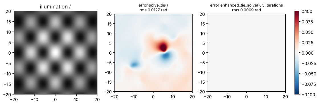
After the first solution, enhanced_tie_solve() computes the residual
\(\partial_z I - \mathrm{TIE}(\varphi)\), solves the TIE for it again and adds the
correction. This helps when the intensity is strongly non-uniform, because
solve_tie() uses an approximation for the term with \(1/I\). We test this with a
strongly structured illumination.
I_struct = I0*(0.55 + 0.45*np.cos(2*np.pi*X/12)*np.cos(2*np.pi*Y/15))
dIdz_struct = TIE.tie(phase, I_struct, x, y, wl)
ph0 = TIE.solve_tie(I_struct, dIdz_struct, x, y, wl, 0.0)
ph_enh = TIE.enhanced_tie_solve(5, I_struct, dIdz_struct, x, y, wl, 0.0, true_phase=None)

fig, axes = plt.subplots(1, 3, figsize=(13, 3.8))
axes[0].imshow(I_struct, extent=ext, cmap="gray"); axes[0].set_title("illumination $I$")
for ax, ph, title in zip(axes[1:], (ph0, ph_enh), ("solve_tie()", "enhanced_tie_solve(), 5 iterations")):
    err = np.where(mask, ph - phase - np.mean((ph - phase)[mask]), np.nan)
    im = ax.imshow(err, extent=ext, cmap="RdBu_r", vmin=-0.1, vmax=0.1)
    ax.set_title(f"error {title}\nrms {rms_error(ph):.4f} rad", fontsize=10)
fig.colorbar(im, ax=axes[1:], fraction=0.03)
for ax in axes:
    ax.set_xlim(-20, 20); ax.set_ylim(-20, 20)
Enanced TIE iteration 1
Enanced TIE iteration 2
Enanced TIE iteration 3
Enanced TIE iteration 4
Enanced TIE iteration 5
References
M. R. Teague, “Deterministic phase retrieval: a Green’s function solution”, J. Opt. Soc. Am. 73, 1434-1441 (1983).
N. Streibl, “Phase imaging by the transport equation of intensity”, Opt. Commun. 49, 6-10 (1984).
D. Paganin and K. A. Nugent, “Noninterferometric phase imaging with partially coherent light”, Phys. Rev. Lett. 80, 2586-2589 (1998).
C. Zuo et al., “Transport of intensity equation: a tutorial”, Opt. Lasers Eng. 135, 106187 (2020).
A. Savitzky and M. J. E. Golay, “Smoothing and differentiation of data by simplified least squares procedures”, Anal. Chem. 36, 1627-1639 (1964).