Phase retrieval: Fienup’s algorithms and phase diversity

Cameras record intensities. The phase of a field, which carries most of the information about an object or about the aberrations of an optical system, is lost. Phase retrieval recovers it from intensity measurements plus some prior knowledge. This notebook treats two classic cases:

1. Support-based phase retrieval (coherent diffractive imaging). We measure only the far-field magnitude \(|\mathcal{F}g|\) of an object \(g\). We also know that \(g\) is confined to a region, its support, and perhaps that it is real and nonnegative. Fienup’s error reduction (ER) and hybrid input-output (HIO) algorithms find \(g\) by alternating projections. Shrink-wrap finds the support along the way. With the detector in the near field, a pyoptics propagator replaces the Fourier transform.

2. Phase diversity (pupil phase retrieval). We measure the PSF of an imaging system at a few known defocus values and recover the pupil phase, i.e. the aberrations. A multi-plane Gerchberg-Saxton iteration and a least squares fit of Zernike coefficients are compared.

pyoptics.phase_retrieval provides:

Function	Purpose
ER(), HIO()	error reduction and hybrid input-output with support, reality and positivity constraints; far field (FT) or near field (any pyoptics propagator to a distance z)
ShrinkWrap, autocorrelation_support()	support update during the iteration, and the initial support from the autocorrelation
fourier_error(), align(), twin()	error metric, and removal of the trivial ambiguities (shift, constant phase, twin image)
diversity_psfs(), defocus_to_waves()	through-focus PSFs of a pupil (paraxial Z4 or exact defocus distances defocus_z), and defocus distance to a Fringe Z4 coefficient
phase_diversity()	pupil phase and Fringe Zernikes from through-focus PSFs (method="fit" or "gs")

All functions return a RetrievalResult with the error history per iteration. The beam shaping counterpart, Gerchberg-Saxton for a phase-only element, lives in pyoptics.ifta (notebook 30).

Conventions: \(\exp(i(\mathbf{k}\cdot\mathbf{r} - \omega t))\); far-field magnitudes are those of fft.FT(). Pupils are sampled on the frequency grid of the PSF grid, as in imaging. Zernike coefficients are Fringe Zernikes in waves, as in litho.

import numpy as np
import matplotlib.pyplot as plt

from pyoptics import phase_retrieval as pr
from pyoptics.bases import FringeZernikes
from pyoptics.fft import FT
from pyoptics.imaging import pupil_coordinates
from pyoptics.processing import CameraNoiser, Scaler
from pyoptics.propagators import rayleigh_sommerfeld_I_TF
from pyoptics.imaging import get_psf
from pyoptics.utils import grid1d

plt.rcParams.update({"figure.dpi": 80, "image.origin": "lower", "font.size": 11})


def show(ax, img, title, cmap="viridis", colorbar=True, **kwargs):
    im = ax.imshow(img, cmap=cmap, **kwargs)
    ax.set_title(title)
    ax.set_xticks([]); ax.set_yticks([])
    if colorbar:
        plt.colorbar(im, ax=ax, fraction=0.046, pad=0.04)
    return im


def log_magnitude(F):
    return np.log10(np.abs(F)/np.abs(F).max() + 1e-6)

1. The phase problem and its trivial ambiguities

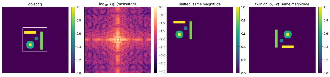
The test object is a real, nonnegative “transmission” image: a few bars and disks of different brightness on a 128 × 128 grid, inside a 48 × 48 pixel region. The grid is more than twice as large as the object, so the far field is oversampled. This is the condition that makes the problem uniquely solvable in 2D, up to the ambiguities discussed next.

Three operations leave \(|\mathcal{F}g|\) unchanged:

• a shift (cyclic, by whole pixels, on a DFT grid),

• a constant phase factor \(e^{i\alpha}\),

• the twin image \(g^*(-x, -y)\).

No algorithm can tell these apart from the magnitude alone. align() undoes them before we compare a reconstruction with the truth.

N = 128
n = np.arange(N) - N//2
X, Y = np.meshgrid(n, n)

obj = np.zeros((N, N))
obj[(np.abs(X + 10) < 12) & (np.abs(Y - 14) < 3)] = 1.0
obj[(np.abs(X - 12) < 3) & (np.abs(Y + 2) < 18)] = 0.8
obj[(X + 10)**2 + (Y + 10)**2 < 8**2] = 0.6
obj[(X + 10)**2 + (Y + 10)**2 < 3**2] = 1.0
obj[(X - 2)**2 + (Y - 2)**2 < 4**2] = 0.4
support = (np.abs(X + 1) < 24) & (np.abs(Y) < 24)   # a box around the object
magnitude = np.abs(FT(obj))

shifted = np.roll(obj, (20, -30), axis=(0, 1))
twinned = pr.twin(obj)
print("max. |F| difference, shifted:", np.max(np.abs(np.abs(FT(shifted)) - magnitude)))
print("max. |F| difference, twin:   ", np.max(np.abs(np.abs(FT(twinned)) - magnitude)))

fig, axes = plt.subplots(1, 4, figsize=(17, 4))
show(axes[0], obj, "object g")
axes[0].contour(support, [0.5], colors="w", linewidths=1)
show(axes[1], log_magnitude(FT(obj)), r"$\log_{10}|\mathcal{F}g|$ (measured)", cmap="magma")
show(axes[2], shifted, "shifted: same magnitude")
show(axes[3], twinned, "twin g*(-x, -y): same magnitude")
plt.tight_layout()

max. |F| difference, shifted: 1.1368683772161603e-13
max. |F| difference, twin:    5.684341886080802e-14

2. Error reduction versus hybrid input-output

Both algorithms first apply the Fourier projection: keep the phase of \(\mathcal{F}g_k\) and impose the measured magnitude, \(g' = \mathcal{F}^{-1}[\,|F|\,e^{i\arg \mathcal{F}g_k}]\). Let \(\gamma\) be the set of pixels where \(g'\) violates the object constraints (outside the support, or negative if positivity is required). Then:

• ER: \(g_{k+1} = g'\) off \(\gamma\) and \(0\) on \(\gamma\), a projection onto the object constraints. Gerchberg-Saxton in disguise: the error \(E_F = \lVert\,|\mathcal{F}g_k| - |F|\,\rVert / \lVert F\rVert\) never increases, but ER stagnates quickly.

• HIO: \(g_{k+1} = g'\) off \(\gamma\) and \(g_k - \beta g'\) on \(\gamma\). The negative feedback keeps pushing the iterate out of the local minima where ER gets stuck. Its \(E_F\) jumps around, so HIO is usually finished with a few ER iterations.

Both start from the same random object inside the support.

er = pr.ER(magnitude, support, N_iter=600, positivity=True, rng=1)
hio = pr.HIO(magnitude, support, beta=0.9, N_iter=550, positivity=True, rng=1)
hio_er = pr.ER(magnitude, support, N_iter=50, start=hio.obj, positivity=True)

er_aligned, er_err = pr.align(er.obj, obj)
hio_aligned, hio_err = pr.align(hio_er.obj, obj)
print(f"ER, 600 iterations:            E_F = {er.errors[-1]:.2e}, object error {er_err:.2e}")
print(f"HIO 550 + ER 50 iterations:    E_F = {hio_er.errors[-1]:.2e}, object error {hio_err:.2e}")

fig = plt.figure(figsize=(17, 4.5))
ax = fig.add_subplot(1, 4, 1)
ax.semilogy(er.errors, label="ER")
ax.semilogy(np.r_[hio.errors, hio_er.errors], label="HIO, then ER")
ax.axvline(550, color="0.6", ls=":")
ax.set_xlabel("iteration"); ax.set_ylabel("Fourier error $E_F$"); ax.legend(); ax.set_title("convergence")
show(fig.add_subplot(1, 4, 2), er_aligned.real, f"ER (aligned), error {er_err:.2f}")
show(fig.add_subplot(1, 4, 3), hio_aligned.real, f"HIO + ER (aligned), error {hio_err:.1e}")
show(fig.add_subplot(1, 4, 4), hio_er.obj, "HIO + ER as returned (shifted/twin)")
plt.tight_layout()

ER, 600 iterations:            E_F = 1.41e-01, object error 6.49e-01
HIO 550 + ER 50 iterations:    E_F = 1.92e-07, object error 7.30e-07

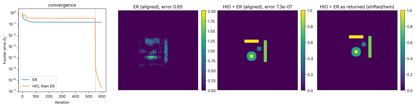
ER is stuck after a few dozen iterations, with a blurred, ghosted image. HIO wanders for a while and then locks onto the solution. The final ER iterations bring \(E_F\) down to round-off. The raw output (right) is a shifted copy or the twin image of the object, depending on the random start.

How much prior knowledge is needed?

Here are HIO + ER runs from five random starts each, with different constraints.

loose = (np.abs(X + 1) < 40) & (np.abs(Y) < 40)
cases = {
    "tight box, positivity": dict(support=support, positivity=True),
    "tight box, real": dict(support=support, real=True),
    "tight box, complex": dict(support=support),
    "loose box, positivity": dict(support=loose, positivity=True),
    "autocorrelation support, positivity": dict(support=pr.autocorrelation_support(magnitude), positivity=True),
}

results = {}
for name, kw in cases.items():
    errs = []
    for seed in range(5):
        r = pr.HIO(magnitude, N_iter=550, rng=seed, **kw)
        kw_er = {key: val for key, val in kw.items() if key != "support"}
        r = pr.ER(magnitude, kw["support"], N_iter=50, start=r.obj, **kw_er)
        errs.append(pr.align(r.obj, obj)[1])
    results[name] = errs
    print(f"{name:38s} object errors: " + ", ".join(f"{e:.1e}" for e in errs))

fig, ax = plt.subplots(figsize=(10, 4))
for i, (name, errs) in enumerate(results.items()):
    ax.semilogy([i]*len(errs), errs, "o", ms=8, alpha=0.7)
ax.set_xticks(range(len(results))); ax.set_xticklabels([s.replace(", ", "\n") for s in results], fontsize=9)
ax.set_ylabel("object error after align()"); ax.axhline(1e-2, color="0.7", ls=":")
ax.set_title("HIO (550) + ER (50), five random starts each")
plt.tight_layout()

tight box, positivity                  object errors: 1.2e-05, 7.3e-07, 1.6e-05, 1.6e-05, 2.1e-06

tight box, real                        object errors: 7.3e-01, 4.5e-01, 8.3e-01, 7.3e-01, 6.6e-01

tight box, complex                     object errors: 6.5e-01, 8.9e-01, 7.8e-01, 9.4e-01, 7.1e-01

loose box, positivity                  object errors: 2.2e-05, 6.4e-01, 1.3e-05, 5.7e-05, 1.5e-05

autocorrelation support, positivity    object errors: 6.2e-06, 9.2e-06, 2.5e-05, 6.7e-06, 3.3e-05

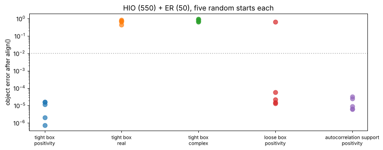
Positivity is the strongest constraint. With it, even the loose autocorrelation support works. Without it, the centrosymmetric box fails in every run. A support that is symmetric under \(\mathbf{x} o -\mathbf{x}\) cannot tell the object from its twin, so the iteration stagnates in a superposition of both (Fienup and Wackerman, JOSA A 3, 1897 (1986)). Tight, asymmetric supports help. Shrink-wrap finds such a support on its own.

3. Unknown support: shrink-wrap

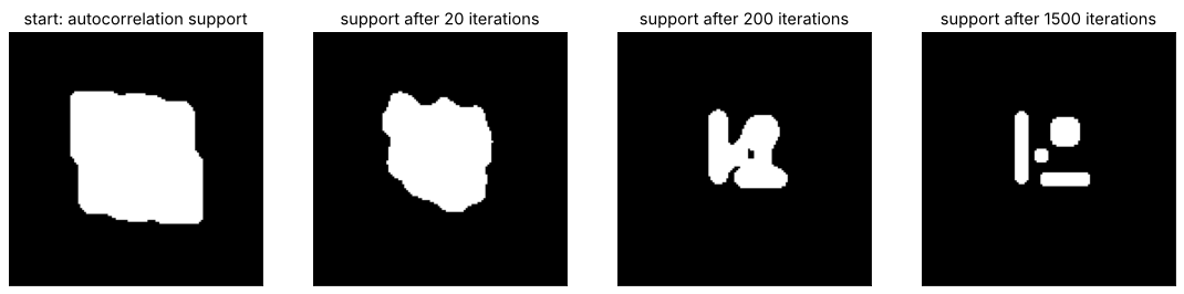
Usually the support is not known. Its autocorrelation is: the inverse FT of \(|F|^2\) is the autocorrelation of \(g\), which is twice as wide as \(g\). autocorrelation_support() thresholds it, which gives a safe but loose start. Shrink-wrap (Marchesini et al. 2003) tightens it during the iteration. Every 20 iterations, the modulus of the current estimate is blurred by a Gaussian and thresholded at 20 % of its maximum to give the new support. The blur shrinks from 3 to 1 pixel as the reconstruction sharpens.

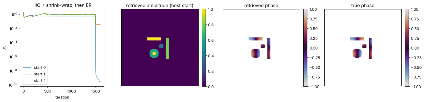
Now the object is complex: the same amplitude with a smooth phase of up to ±0.8 rad, so neither positivity nor reality can help. Complex objects are much harder. HIO can stagnate in a mixture of the object and its twin. The usual remedy is to run a few random starts and keep the one with the lowest Fourier error, which needs no knowledge of the true object. A callback records snapshots of the support.

phase_obj = 0.8*np.cos(X/6.0)*np.sin(Y/7.0)
cobj = obj*np.exp(1j*phase_obj)
cmagnitude = np.abs(FT(cobj))

runs = []
for seed in range(3):
    snapshots = {}
    record = lambda i, g, s, snapshots=snapshots: snapshots.update({i: s.copy()}) if i in (20, 200, 1500) else None
    r = pr.HIO(cmagnitude, None, N_iter=1500, shrinkwrap=pr.ShrinkWrap(every=20, sigma=3.0, sigma_min=1.0, decay=0.95, threshold=0.2),
               rng=seed, callback=record)
    final = pr.ER(cmagnitude, r.support, N_iter=100, start=r.obj)
    runs.append((final.errors[-1], seed, r, final, snapshots))
    print(f"start {seed}: E_F = {final.errors[-1]:.1e}, object error (needs the truth) {pr.align(final.obj, cobj)[1]:.1e}")

E_F, seed, r, final, snapshots = min(runs, key=lambda run: run[0])
aligned, err = pr.align(final.obj, cobj)
print(f"best start {seed}: object error {err:.1e}; support pixels {r.support.sum()} (object: {(obj > 0).sum()})")

fig, axes = plt.subplots(1, 4, figsize=(17, 4))
show(axes[0], pr.autocorrelation_support(cmagnitude), "start: autocorrelation support", cmap="gray", colorbar=False)
for ax, i in zip(axes[1:], sorted(snapshots)):
    show(ax, snapshots[i], f"support after {i} iterations", cmap="gray", colorbar=False)

fig, axes = plt.subplots(1, 4, figsize=(17, 4.2))
for E, s_, r_, f_, _ in runs:
    axes[0].semilogy(np.r_[r_.errors, f_.errors], lw=1, label=f"start {s_}")
axes[0].set_xlabel("iteration"); axes[0].set_ylabel("$E_F$"); axes[0].legend(); axes[0].set_title("HIO + shrink-wrap, then ER")
lit = np.abs(cobj) > 0.05
show(axes[1], np.abs(aligned), "retrieved amplitude (best start)")
show(axes[2], np.where(np.abs(aligned) > 0.05, np.angle(aligned), np.nan), "retrieved phase", cmap="twilight", vmin=-1, vmax=1)
show(axes[3], np.where(lit, np.angle(cobj), np.nan), "true phase", cmap="twilight", vmin=-1, vmax=1)
plt.tight_layout()

start 0: E_F = 1.9e-10, object error (needs the truth) 1.1e-09

start 1: E_F = 3.6e-02, object error (needs the truth) 8.5e-02

start 2: E_F = 4.1e-02, object error (needs the truth) 1.0e-01
best start 0: object error 1.1e-09; support pixels 668 (object: 528)

4. Near field: a propagator instead of the Fourier transform

Nothing in ER and HIO requires the far field. The algorithms only need a transform from the object to the detector and its inverse. With z (and the grid and wavelength), the Fourier transforms are replaced by a pyoptics propagator to the distance z and back by -z. By default this is the angular spectrum method propagators.rayleigh_sommerfeld_I_TF, but any grid-preserving propagator can be passed as propagator. This is Fresnel coherent diffractive imaging.

The Fresnel kernel \(\exp(i k r^2/2z)\) is not symmetric under \(g(\mathbf{x}) \to g^*(-\mathbf{x})\), so the twin image no longer has the same measured magnitude. The same holds for shifts. Only the constant phase remains ambiguous. We test this on the case that failed in the far field above: the real object in the centrosymmetric box, with the reality constraint but without positivity. The grid now has a physical pitch of 1 µm, with λ = 0.5 µm. The errors over four random starts are plotted against the Fresnel number \(N_F = a^2/(\lambda z)\) of the object half width \(a = 24\) µm.

wl_cdi = 0.5
x_cdi = n.astype(float)               # 1 um pixels: no evanescent waves on the grid
a = 24.0
distances = [100.0, 200.0, 300.0, 600.0, 1000.0]


def run_near(z, seed):
    m = np.abs(rayleigh_sommerfeld_I_TF(obj, x_cdi, x_cdi, z, wl_cdi)[0])
    kw = dict(z=z, x=x_cdi, y=x_cdi, wavelength=wl_cdi, real=True)
    r = pr.HIO(m, support, N_iter=400, rng=seed, **kw)
    return m, pr.ER(m, support, N_iter=100, start=r.obj, **kw)


def near_error(rec):
    sign = np.sign(np.sum(rec*obj))   # the constant phase of a real object
    return np.linalg.norm(sign*rec - obj)/np.linalg.norm(obj)


far_errors, far_results = [], []
for seed in range(4):
    r = pr.HIO(magnitude, support, N_iter=400, rng=seed, real=True)
    r = pr.ER(magnitude, support, N_iter=100, start=r.obj, real=True)
    far_errors.append(pr.align(r.obj, obj)[1])
    far_results.append(r)

near_errors, examples = {}, {}
for z in distances:
    errs = []
    for seed in range(4):
        m, r = run_near(z, seed)
        errs.append(near_error(r.obj))
        examples.setdefault(z, (m, r))
    near_errors[z] = errs
    print(f"z = {z:6.0f} um, N_F = {a**2/(wl_cdi*z):5.2f}: errors " + ", ".join(f"{e:.0e}" for e in errs))
print("far field:                    errors " + ", ".join(f"{e:.0e}" for e in far_errors))

fig, axes = plt.subplots(1, 4, figsize=(18, 4.2))
ax = axes[0]
for z, errs in near_errors.items():
    ax.semilogy([a**2/(wl_cdi*z)]*len(errs), errs, "o", color="C0", alpha=0.7)
ax.semilogy([0.2]*len(far_errors), far_errors, "s", color="C3", alpha=0.7, label="far field")
ax.set_xscale("log"); ax.set_xlabel("Fresnel number $N_F$ (far field at the left)"); ax.set_ylabel("object error")
ax.set_title("real object, box, no positivity"); ax.legend()
m, r = examples[300.0]
show(axes[1], m**2, "near-field intensity, z = 300 µm", cmap="magma")
show(axes[2], np.sign(np.sum(r.obj*obj))*r.obj, f"retrieved, z = 300 µm, error {near_error(r.obj):.0e}")
show(axes[3], pr.align(far_results[0].obj, obj)[0].real, "far field, same constraints")
plt.tight_layout()

z =    100 um, N_F = 11.52: errors 5e-01, 5e-01, 4e-01, 5e-01

z =    200 um, N_F =  5.76: errors 9e-01, 9e-01, 9e-01, 9e-01

z =    300 um, N_F =  3.84: errors 1e-06, 1e-06, 9e-07, 9e-07

z =    600 um, N_F =  1.92: errors 2e-09, 2e-09, 2e-09, 3e-09

z =   1000 um, N_F =  1.15: errors 6e-08, 4e-08, 6e-08, 3e-08
far field:                    errors 7e-01, 5e-01, 9e-01, 7e-01

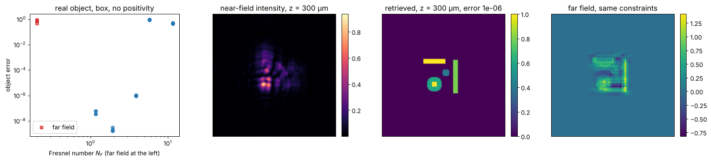
In the far field, all runs stagnate in a mixture of object and twin. At Fresnel numbers of about 1 to 4, the near-field data give the object to round-off from every start, with no shift or twin to remove. Very close to the object (large \(N_F\)) retrieval fails again. There the intensity is almost the modulus of the object itself, and the phase has had no distance to turn into intensity (compare TIE in notebook 29). The near field is no cure-all either. For the complex object in the loose box, we saw no reliable success at any distance; it still needs a tight support or shrink-wrap.

For real data, keep \(z\) below the critical distance of the angular spectrum method, \(N\,\Delta x^2/\lambda\) (256 µm here; propagators.suggest_N_critical()), or pass functools.partial(propagators.propagate_padded, ...) as the propagator. Otherwise the cyclic convolution wraps light around the window. The simulated data here use the same propagator as the retrieval, so they are consistent at any \(z\).

5. Noise

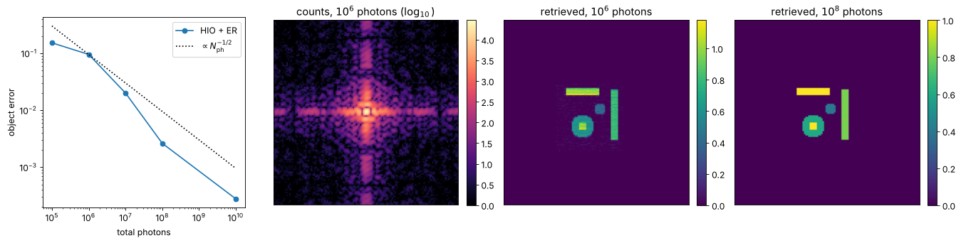
A real diffraction pattern is a photon count. We scale \(|F|^2\) to a given total photon number, add Poisson noise with processing.CameraNoiser, and retrieve from the square root of the counts. With the default ER/HIO there is no noise model. The reconstruction error decreases roughly like \(N_\mathrm{ph}^{-1/2}\).

noiser = CameraNoiser("poisson", rng=7)
photons = [1e5, 1e6, 1e7, 1e8, 1e10]
noise_errors, examples = [], {}
for N_ph in photons:
    I = Scaler(N_ph, measure="total")(magnitude**2)
    counts = noiser(I)
    r = pr.HIO(np.sqrt(counts), support, N_iter=550, positivity=True, rng=1)
    r = pr.ER(np.sqrt(counts), support, N_iter=50, start=r.obj, positivity=True)
    rec = r.obj*np.sqrt(np.sum(magnitude**2)/np.sum(counts))   # back to the scale of obj
    aligned, err = pr.align(rec, obj)
    noise_errors.append(err)
    examples[N_ph] = (counts, aligned.real)

fig, axes = plt.subplots(1, 4, figsize=(17, 4.2))
axes[0].loglog(photons, noise_errors, "o-", label="HIO + ER")
axes[0].loglog(photons, noise_errors[1]*np.sqrt(photons[1]/np.array(photons)), "k:", label=r"$\propto N_\mathrm{ph}^{-1/2}$")
axes[0].set_xlabel("total photons"); axes[0].set_ylabel("object error"); axes[0].legend()
show(axes[1], np.log10(examples[1e6][0] + 1), r"counts, $10^6$ photons ($\log_{10}$)", cmap="magma")
show(axes[2], examples[1e6][1], r"retrieved, $10^6$ photons")
show(axes[3], examples[1e8][1], r"retrieved, $10^8$ photons")
plt.tight_layout()

6. Pupil phase from through-focus PSFs: phase diversity

Now consider an imaging system with numerical aperture NA and an unknown pupil phase \(\varphi(P_x, P_y)\). The amplitude PSF is the inverse FT of the pupil function \(P = |P|\,e^{i\varphi}\), exactly as in imaging.get_psf(). The pupil amplitude is known (a clear circle here). A single in-focus PSF is not enough: \(\varphi(\mathbf{P})\) and \(-\varphi(-\mathbf{P})\) give the same intensity, so the sign of all even aberrations (defocus, astigmatism, spherical) is undetermined.

The remedy is phase diversity. We also record PSFs with a known extra defocus, which adds \(2\pi c_4 Z_4\) with the Fringe Zernike \(Z_4 = 2P^2 - 1\) to the pupil phase. defocus_to_waves() converts an axial shift \(\Delta z\) of the observation plane into \(c_4\). Paraxially, \(k_z \approx k - k\,\mathrm{NA}^2 P^2/2\), so \(c_4 = -k\,\Delta z\,\mathrm{NA}^2/(8\pi)\). This is checked here against an angular spectrum propagation of an aberrated PSF.

Alternatively, defocus_z gives the diversity as physical distances. The pupil is then multiplied by the exact angular spectrum propagator \(\exp(i(k_z - k)\Delta z)\). That is the same as calling propagators.rayleigh_sommerfeld_I_TF() on the in-focus PSF, but it costs one FFT instead of two (see section 8).

wl = 0.5                    # um
k = 2*np.pi/wl
NA = 0.1
N_chk = 256
L_chk = N_chk*wl/(4*NA)
x_chk = grid1d(-L_chk/2, L_chk/2, N_chk)
spherical = lambda P_x, P_y: 2*np.pi*0.3*(6*(P_x**2 + P_y**2)**2 - 6*(P_x**2 + P_y**2) + 1)   # 0.3 waves Z9
psf_focus = get_psf(x_chk, x_chk, NA, k, phase=spherical)

fig, axes = plt.subplots(1, 4, figsize=(17, 4))
crop = slice(N_chk//2 - 14, N_chk//2 + 15)
for i, dz in enumerate((-100.0, 100.0)):
    I_prop = np.abs(rayleigh_sommerfeld_I_TF(psf_focus, x_chk, x_chk, dz, wl)[0])**2
    I_prop /= I_prop.sum()
    c4 = pr.defocus_to_waves(dz, NA, k)
    I_model = pr.diversity_psfs(x_chk, x_chk, NA, k, [c4], phase=spherical)[0]
    print(f"dz = {dz:+.0f} um -> c4 = {c4:+.3f} waves; max. deviation from propagation: "
          f"{np.max(np.abs(I_prop - I_model))/I_prop.max():.1e} of the peak")
    show(axes[2*i], I_prop[crop, crop], f"propagated, dz = {dz:+.0f} µm", cmap="magma")
    show(axes[2*i + 1], I_model[crop, crop], f"pupil with c4 = {c4:+.2f} waves", cmap="magma")
plt.tight_layout()

dz = -100 um -> c4 = +0.500 waves; max. deviation from propagation: 1.6e-03 of the peak
dz = +100 um -> c4 = -0.500 waves; max. deviation from propagation: 1.6e-03 of the peak

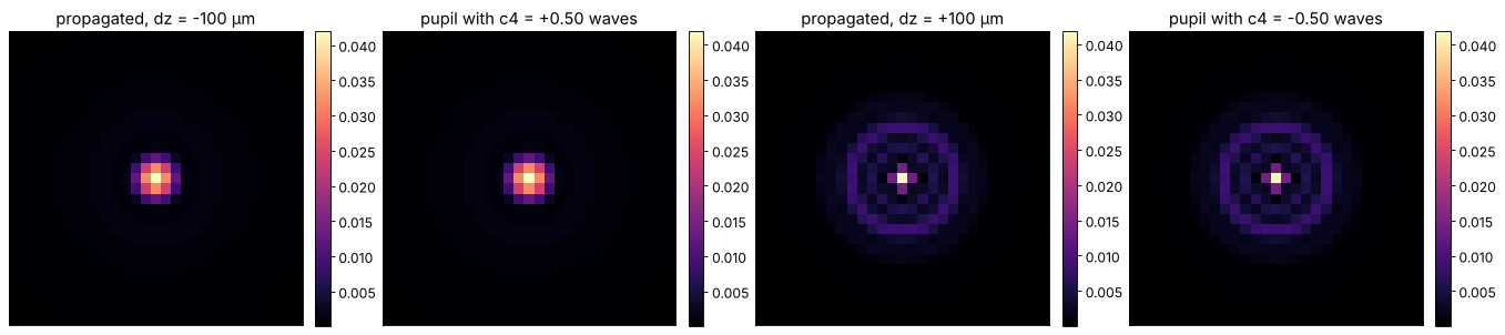
The small residual is the non-paraxial part of \(k_z\). Note how different the two sides of focus look with spherical aberration. This asymmetry is what phase diversity exploits.

The test system

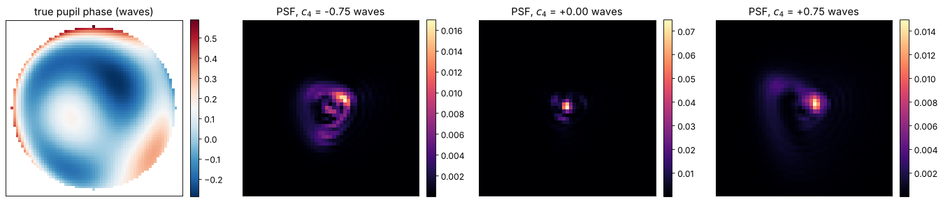
NA = 0.25, λ = 0.5 µm, a 128 × 128 PSF grid with \(\Delta x = \lambda/(4\,\mathrm{NA})\) (Nyquist for the intensity). The pupil radius is then 32 pixels. The unknown pupil phase is a random combination of Fringe Zernikes 2 to 15 with about 0.15 waves rms. Three PSFs are recorded at \(c_4 = -0.75, 0, +0.75\) waves.

NA = 0.25
N_psf = 128
L = N_psf*wl/(4*NA)
x = grid1d(-L/2, L/2, N_psf)
P_x, P_y = pupil_coordinates(x, x, NA, k)
inside = P_x**2 + P_y**2 <= 1
zern = FringeZernikes(P_x[0], P_y[:, 0])
Z = lambda j: zern.eval_single_scattered(P_x, P_y, j)
pupil_crop = slice(N_psf//2 - 34, N_psf//2 + 35)
psf_crop = slice(N_psf//2 - 24, N_psf//2 + 25)


def phase_from(coeffs):
    return 2*np.pi*sum(c*Z(j) for j, c in coeffs.items())*inside


def rms_waves(phase, reference):
    d = (phase - reference)[inside]
    d -= d.mean()
    return np.sqrt(np.mean(d**2))/(2*np.pi)


rng = np.random.default_rng(0)
true = {j: rng.normal(0, 0.4)/np.sqrt(j) for j in range(2, 16)}
true_phase = phase_from(true)
print(f"true pupil phase: {rms_waves(true_phase, 0*true_phase):.3f} waves rms")

defocus = [-0.75, 0.0, 0.75]
psfs = pr.diversity_psfs(x, x, NA, k, defocus, phase=true_phase)

fig, axes = plt.subplots(1, 4, figsize=(17, 4))
show(axes[0], np.where(inside, true_phase/(2*np.pi), np.nan)[pupil_crop, pupil_crop], "true pupil phase (waves)", cmap="RdBu_r")
for ax, d, p in zip(axes[1:], defocus, psfs):
    show(ax, p[psf_crop, psf_crop], f"PSF, $c_4$ = {d:+.2f} waves", cmap="magma")
plt.tight_layout()

true pupil phase: 0.156 waves rms

Why one in-focus PSF is not enough

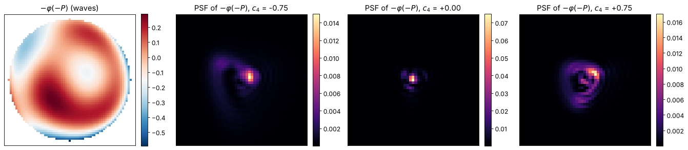
Replace \(\varphi(\mathbf{P})\) with \(-\varphi(-\mathbf{P})\), i.e. flip the sign of the even Zernikes and keep the odd ones. The amplitude PSF becomes its complex conjugate, \(h \to h^*\), so the in-focus intensity does not change at all. Defocus is even, so the defocused PSFs swap sides of focus: the PSF at \(+c_4\) becomes the PSF at \(-c_4\). A fit to the in-focus PSF alone has no way to choose, and here it lands exactly on the wrong one.

flipped = -true_phase[::-1, ::-1]
flipped = np.roll(flipped, (1, 1), axis=(0, 1))*inside     # -phi(-P) on the centred grid
psf_flip = pr.diversity_psfs(x, x, NA, k, defocus, phase=flipped)
print("in-focus PSFs equal:", np.allclose(psfs[1], psf_flip[1]))
print("defocused PSFs swapped:", np.allclose(psfs[0], psf_flip[2]) and np.allclose(psfs[2], psf_flip[0]))

fig, axes = plt.subplots(1, 4, figsize=(17, 4))
show(axes[0], np.where(inside, flipped/(2*np.pi), np.nan)[pupil_crop, pupil_crop], r"$-\varphi(-P)$ (waves)", cmap="RdBu_r")
for ax, d, p in zip(axes[1:], defocus, psf_flip):
    show(ax, p[psf_crop, psf_crop], f"PSF of $-\\varphi(-P)$, $c_4$ = {d:+.2f}", cmap="magma")
plt.tight_layout()

single = pr.phase_diversity(psfs[1:2], [0.0], x, x, NA, k, n_zernike=15)
print(f"fit to the in-focus PSF alone: residual phase error {rms_waves(single.phase, true_phase):.3f} waves rms, "
      f"vs. the flipped solution {rms_waves(single.phase, flipped):.3f} waves rms")

in-focus PSFs equal: True
defocused PSFs swapped: True

fit to the in-focus PSF alone: residual phase error 0.204 waves rms, vs. the flipped solution 0.000 waves rms

Retrieval: Zernike fit versus multi-plane Gerchberg-Saxton

• method="fit" models the three intensities with Fringe Zernikes 2 to 15 and minimises the squared intensity residuals with scipy.optimize.least_squares, using the analytic Jacobian. The energy of the model PSF does not depend on the phase (Parseval), so each measured PSF is simply normalised to it. No scale factors need fitting.

• method="gs" (Misell’s multi-plane Gerchberg-Saxton) cycles through the planes. In each, it propagates the current pupil to the PSF, imposes the measured modulus, propagates back and removes the known defocus, then imposes the known pupil amplitude. It needs no basis. Afterwards its phase is unwrapped (unwrap.unwrap_quality_guided()) and fitted with Zernikes.

The error is the normalised rms deviation of the model amplitudes \(\sqrt{I}\) from the measured ones.

import time

t0 = time.perf_counter()
fit = pr.phase_diversity(psfs, defocus, x, x, NA, k, n_zernike=15, method="fit")
t_fit = time.perf_counter() - t0
t0 = time.perf_counter()
gs = pr.phase_diversity(psfs, defocus, x, x, NA, k, n_zernike=15, method="gs", N_iter=300)
t_gs = time.perf_counter() - t0
print(f"fit: {rms_waves(fit.phase, true_phase):.1e} waves rms error, {len(fit.errors)} evaluations, {t_fit:.2f} s")
print(f"gs:  {rms_waves(gs.phase, true_phase):.1e} waves rms error, {len(gs.errors)} iterations, {t_gs:.2f} s")

fig = plt.figure(figsize=(17, 4.5))
ax = fig.add_subplot(1, 3, 1)
ax.semilogy(fit.errors, "o-", label="Zernike fit (per evaluation)")
ax.semilogy(gs.errors, label="multi-plane GS (per iteration)")
ax.set_xlabel("evaluation / iteration"); ax.set_ylabel("amplitude error"); ax.legend(); ax.set_title("convergence")

ax = fig.add_subplot(1, 3, (2, 3))
j = np.arange(2, 16)
ax.bar(j - 0.27, [true[i] for i in j], 0.27, label="true")
ax.bar(j, [fit.zernikes[i] for i in j], 0.27, label="fit")
ax.bar(j + 0.27, [gs.zernikes[i] for i in j], 0.27, label="GS")
ax.set_xticks(j); ax.set_xlabel("Fringe Zernike j"); ax.set_ylabel("coefficient (waves)"); ax.legend()
ax.set_title("retrieved Zernike coefficients")
plt.tight_layout()

fit: 3.8e-17 waves rms error, 7 evaluations, 0.95 s
gs:  3.6e-17 waves rms error, 300 iterations, 1.90 s

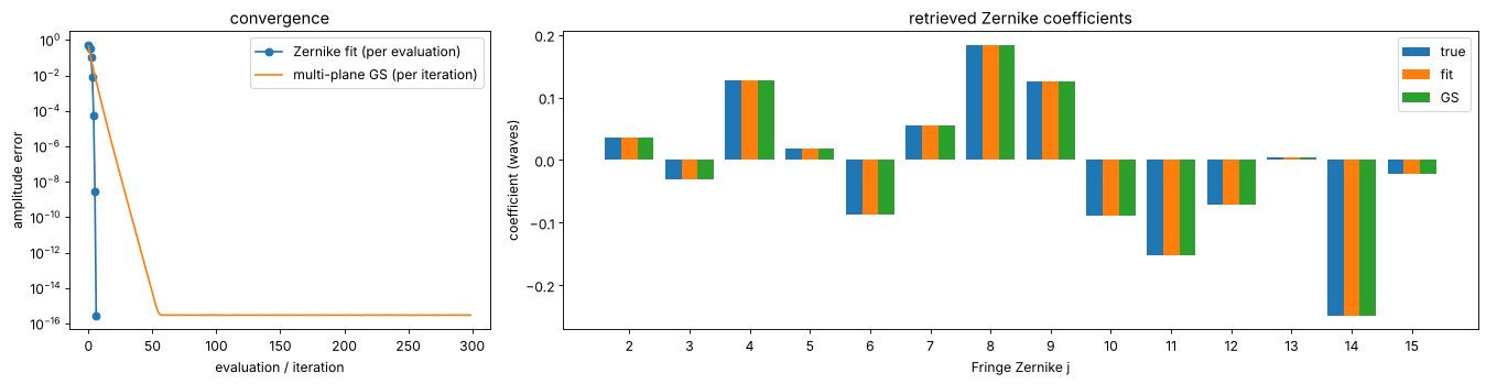
Without noise, both recover the phase to round-off. The fit needs fewer than ten evaluations, but each one includes the Jacobian (one FFT per plane and Zernike). GS needs about 50 cheap iterations here (two FFTs per plane). Its convergence slows down for larger aberrations, the familiar behaviour of alternating projections. The fit starts from zero and still converged for random aberrations up to about half a wave rms in our trials. GS needs no basis, so it can also capture phase structure beyond the Zernikes in use, such as a segment step or a zone error. Its result can then be passed as start to a fit.

7. Noise and the amount of diversity

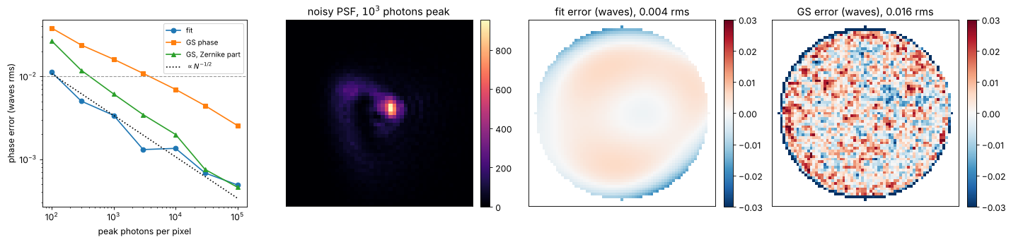
Next, Poisson noise with CameraNoiser. Each PSF is scaled to a given peak photon count per pixel. As expected, the error falls like \(N_\mathrm{ph}^{-1/2}\). The fit is better than GS because it uses the known phase structure (14 parameters instead of about 3200 pupil pixels). Fitting Zernikes to the GS phase recovers much of that advantage: the noise in the pupil pixels is mostly of high spatial frequency and averages out in the Zernike projection.

noiser = CameraNoiser("poisson", rng=11)
peaks = [1e2, 3e2, 1e3, 3e3, 1e4, 3e4, 1e5]
err_fit, err_gs, err_gs_z = [], [], []
for peak in peaks:
    noisy = np.array([noiser(Scaler(peak)(p)) for p in psfs])
    f = pr.phase_diversity(noisy, defocus, x, x, NA, k, n_zernike=15, method="fit")
    g = pr.phase_diversity(noisy, defocus, x, x, NA, k, n_zernike=15, method="gs", N_iter=100)
    err_fit.append(rms_waves(f.phase, true_phase))
    err_gs.append(rms_waves(g.phase, true_phase))
    err_gs_z.append(rms_waves(phase_from(g.zernikes), true_phase))

noisy_1e3 = np.array([noiser(Scaler(1e3)(p)) for p in psfs])
f_1e3 = pr.phase_diversity(noisy_1e3, defocus, x, x, NA, k, n_zernike=15, method="fit")
g_1e3 = pr.phase_diversity(noisy_1e3, defocus, x, x, NA, k, n_zernike=15, method="gs", N_iter=100)

fig, axes = plt.subplots(1, 4, figsize=(18, 4.2))
axes[0].loglog(peaks, err_fit, "o-", label="fit")
axes[0].loglog(peaks, err_gs, "s-", label="GS phase")
axes[0].loglog(peaks, err_gs_z, "^-", label="GS, Zernike part")
axes[0].loglog(peaks, err_fit[2]*np.sqrt(peaks[2]/np.array(peaks)), "k:", label=r"$\propto N^{-1/2}$")
axes[0].axhline(0.01, color="0.6", ls="--", lw=1)
axes[0].set_xlabel("peak photons per pixel"); axes[0].set_ylabel("phase error (waves rms)"); axes[0].legend(fontsize=9)
show(axes[1], noisy_1e3[2][psf_crop, psf_crop], "noisy PSF, $10^3$ photons peak", cmap="magma")
lim = 0.03
show(axes[2], np.where(inside, (f_1e3.phase - true_phase)/(2*np.pi), np.nan)[pupil_crop, pupil_crop],
     f"fit error (waves), {rms_waves(f_1e3.phase, true_phase):.3f} rms", cmap="RdBu_r", vmin=-lim, vmax=lim)
d_gs = (g_1e3.phase - true_phase)
d_gs -= d_gs[inside].mean()
show(axes[3], np.where(inside, d_gs/(2*np.pi), np.nan)[pupil_crop, pupil_crop],
     f"GS error (waves), {rms_waves(g_1e3.phase, true_phase):.3f} rms", cmap="RdBu_r", vmin=-lim, vmax=lim)
plt.tight_layout()

How much defocus should the diversity planes have? Too little, and the planes carry nearly the same information as the focus. Too much, and the light spreads over many pixels, which lowers the signal per pixel at a fixed peak count. A sweep with \(\pm c_4\) around focus at \(10^3\) photons peak (each point averaged over three noise realisations):

amounts = [0.1, 0.25, 0.5, 0.75, 1.0, 1.5, 2.0]
mean_err = []
for a in amounts:
    planes = [-a, 0.0, a]
    clean = pr.diversity_psfs(x, x, NA, k, planes, phase=true_phase)
    errs = []
    for rep in range(3):
        noisy = np.array([noiser(Scaler(1e3)(p)) for p in clean])
        errs.append(rms_waves(pr.phase_diversity(noisy, planes, x, x, NA, k, n_zernike=15).phase, true_phase))
    mean_err.append(np.mean(errs))

fig, ax = plt.subplots(figsize=(7, 4))
ax.plot(amounts, mean_err, "o-")
ax.set_xlabel(r"diversity $\pm c_4$ (waves)"); ax.set_ylabel("phase error (waves rms)")
ax.set_title(r"three planes $-c_4, 0, +c_4$; $10^3$ photons peak")
ax.set_ylim(0, None)
plt.tight_layout()

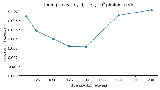
A diversity of about half a wave to one wave of \(c_4\) is best here. That is one to two waves of peak-to-valley defocus, or \(\Delta z = 4\lambda c_4/\mathrm{NA}^2 \approx 2\) to \(4\,\lambda/\mathrm{NA}^2\) (defocus_to_waves() converts). Larger values still work, at a gradually higher error. In practice the diversity defocus itself is known only to the accuracy of the focus stage. A natural extension is to include it as a fit parameter.

8. High NA: exact defocus instead of the paraxial Z4

The paraxial model of defocus, a pure \(Z_4\), misses the higher terms of \(k_z = \sqrt{k^2 - k_\perp^2}\): spherical aberration of all orders, which grows like \(\mathrm{NA}^4 \Delta z\). With defocus_z, the diversity is applied exactly. Here the PSFs are simulated with exact defocus at the same Z4-equivalent diversity (\(\pm 0.75\) waves paraxially) for several NA. They are then retrieved once with the exact model and once with the paraxial model, using the \(c_4\) from defocus_to_waves().

NAs = [0.1, 0.25, 0.4, 0.55, 0.7, 0.85]
err_exact, err_parax = [], []
for NA_i in NAs:
    L_i = N_psf*wl/(4*NA_i)
    x_i = grid1d(-L_i/2, L_i/2, N_psf)
    Px_i, Py_i = pupil_coordinates(x_i, x_i, NA_i, k)
    inside_i = Px_i**2 + Py_i**2 <= 1
    zern_i = FringeZernikes(Px_i[0], Py_i[:, 0])
    phase_i = 2*np.pi*sum(c*zern_i.eval_single_scattered(Px_i, Py_i, j) for j, c in true.items())*inside_i
    dz = 0.75*4*wl/NA_i**2
    planes = np.array([-dz, 0.0, dz])
    psfs_i = pr.diversity_psfs(x_i, x_i, NA_i, k, phase=phase_i, defocus_z=planes)
    for method_errors, kwargs in ((err_exact, dict(defocus_waves=None, defocus_z=planes)),
                                  (err_parax, dict(defocus_waves=pr.defocus_to_waves(planes, NA_i, k)))):
        r = pr.phase_diversity(psfs_i, x=x_i, y=x_i, NA=NA_i, k=k, **kwargs)
        d = (r.phase - phase_i)[inside_i]
        method_errors.append(np.sqrt(np.mean((d - d.mean())**2))/(2*np.pi))

fig, ax = plt.subplots(figsize=(7, 4))
ax.semilogy(NAs, err_parax, "o-", label="paraxial model (Z4)")
ax.semilogy(NAs, np.maximum(err_exact, 1e-17), "s-", label="exact model (defocus_z)")
ax.axhline(0.01, color="0.6", ls="--", lw=1)
ax.set_xlabel("NA"); ax.set_ylabel("phase error (waves rms)"); ax.legend()
ax.set_title(r"diversity $\Delta z = \pm 3\lambda/\mathrm{NA}^2$, noise free")
plt.tight_layout()

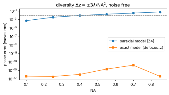
The exact model recovers the phase to round-off at any NA. The paraxial model passes λ/100 at an NA of about 0.4. Above that, the neglected defocus terms end up in the retrieved spherical aberration and defocus.

Summary

• ER() and HIO() retrieve an object from its Fourier magnitude. HIO escapes the stagnation of ER, and a few ER iterations polish the result. Tight supports and positivity make the problem much better conditioned. ShrinkWrap finds the support when only the autocorrelation is known.

• The result is unique only up to a shift, a constant phase and the twin image. align() removes these for comparisons.

• With z, the detector is in the near field, and a pyoptics propagator replaces the Fourier transform. At Fresnel numbers of about 1 to 4, this removes the twin and shift ambiguities. It even solves the centrosymmetric-support case without positivity.

• A single in-focus PSF cannot fix the sign of the even aberrations. Known defocus diversity resolves it, and phase_diversity() then recovers the pupil phase to below λ/100 rms without noise (defocus_z applies the diversity exactly, which matters above an NA of about 0.4). method="fit" is fast and noise robust for Zernike-type aberrations. method="gs" is basis free and can seed the fit.

References

• R. W. Gerchberg and W. O. Saxton, “A practical algorithm for the determination of phase from image and diffraction plane pictures”, Optik 35, 237-246 (1972).

• J. R. Fienup, “Reconstruction of an object from the modulus of its Fourier transform”, Opt. Lett. 3, 27-29 (1978).

• J. R. Fienup, “Phase retrieval algorithms: a comparison”, Appl. Opt. 21, 2758-2769 (1982).

• J. R. Fienup and C. C. Wackerman, “Phase-retrieval stagnation problems and solutions”, J. Opt. Soc. Am. A 3, 1897-1907 (1986).

• S. Marchesini, H. He, H. N. Chapman, S. P. Hau-Riege, A. Noy, M. R. Howells, U. Weierstall and J. C. H. Spence, “X-ray image reconstruction from a diffraction pattern alone”, Phys. Rev. B 68, 140101 (2003).

• G. J. Williams, H. M. Quiney, B. B. Dhal, C. Q. Tran, K. A. Nugent, A. G. Peele, D. Paterson and M. D. de Jonge, “Fresnel coherent diffractive imaging”, Phys. Rev. Lett. 97, 025506 (2006).

• D. L. Misell, “An examination of an iterative method for the solution of the phase problem in optics and electron optics: I. Test calculations”, J. Phys. D 6, 2200-2216 (1973).

• R. A. Gonsalves, “Phase retrieval and diversity in adaptive optics”, Opt. Eng. 21, 829-832 (1982).

• J. R. Fienup, J. C. Marron, T. J. Schulz and J. H. Seldin, “Hubble Space Telescope characterized by using phase-retrieval algorithms”, Appl. Opt. 32, 1747-1767 (1993).