Mode analysis and fibre modes

A coherent beam can always be written as a sum of the paraxial Hermite-Gaussian (HG) or Laguerre-Gaussian (LG) modes of some basis. The mode content tells us how “Gaussian” a beam is, how it will propagate, and how much of it a single mode fibre will accept. This notebook shows the tools of pyoptics.modes:

1. Decomposition into HG and LG modes: power fractions, the choice of the basis waist, a fitted basis.

2. A spiral phase plate in front of a Gaussian beam, against the analytic LG mode content.

3. M² from the mode content, checked against an ISO 11146 caustic measurement with beam_quality.

4. LP modes of a weakly guiding step-index fibre: dispersion diagram, cutoffs, mode fields, the Marcuse approximation of the mode field radius.

5. Coupling into fibres: an arbitrary field into LP01 (generalizing abcd.coupling_efficiency()), misalignment sweeps, aberrated beams, and the excitation of higher modes in a few-mode fibre.

Lengths are in µm. All fields use the pyoptics convention \(\exp(i(\mathbf{k}\cdot\mathbf{r} - \omega t))\).

from math import factorial, gamma, pi, sqrt

import numpy as np
import matplotlib.pyplot as plt
from scipy.integrate import quad
from scipy.optimize import minimize_scalar

from pyoptics import abcd, modes
from pyoptics.beam_quality import beam_widths, fit_caustic
from pyoptics.utils import grid2d

plt.rcParams.update({"figure.dpi": 80, "image.origin": "lower", "font.size": 11})


def show(ax, img, title, extent=None, cmap="viridis", colorbar=True, **kwargs):
    im = ax.imshow(img, cmap=cmap, extent=extent, **kwargs)
    ax.set_title(title)
    if colorbar:
        plt.colorbar(im, ax=ax, fraction=0.046, pad=0.04)
    return im


def show_phase(ax, field, title, extent=None, threshold=1E-3):
    # phase where the intensity is above threshold of its maximum, else white
    I = np.abs(field)**2
    phase = np.ma.masked_where(I < threshold*I.max(), np.angle(field))
    return show(ax, phase, title, extent, cmap="twilight", vmin=-np.pi, vmax=np.pi)


def bars(ax, decomposition, n_show=12, title=""):
    # the strongest modes of a decomposition as a bar chart
    fractions = sorted(decomposition.power_fractions.items(), key=lambda kv: -kv[1])[:n_show]
    labels = [("HG" if decomposition.family == "hg" else "LG") + "$_{%d,%d}$" % key for key, _ in fractions]
    ax.bar(range(len(fractions)), [f for _, f in fractions], color="C0")
    ax.set_xticks(range(len(fractions)))
    ax.set_xticklabels(labels, rotation=60)
    ax.set_ylabel("power fraction")
    ax.set_title(title)

1. Decomposition into HG and LG modes

decompose_hg(field, x, y, w0, wavelength, z, max_order) projects a field onto the modes \(u_{lm}\) of beams.gauss_hermite() with waist \(w_0\), a distance \(z\) behind the waist, up to the order \(N = l + m \le\) max_order. decompose_lg() does the same with the LG modes \(u_{pl}\) of beams.gauss_laguerre(), \(N = 2p + |l|\). Both sets of modes of the orders \(0 \dots N\) span the same space, so a field has the same power per order in both bases. The modes are normalized numerically on the grid, and \(|c_j|^2/P\) is the fraction of the power \(P\) in mode \(j\).

The modes contain the Gouy phase. The coefficients therefore don’t change when the field and the basis propagate together, and the reconstruction \(\sum_j c_j u_j\) can be evaluated at any \(z\).

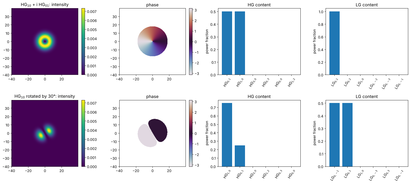
First example: the “donut” \(\mathrm{HG}_{10} + i\,\mathrm{HG}_{01}\) is the single mode \(\mathrm{LG}_{0,+1}\), while a rotated \(\mathrm{HG}_{10}\) is a sum of two HG modes but also two LG modes.

wl = 1.0
x, y, X, Y = grid2d(-40, 40, -40, 40, 256)
extent = [x[0], x[-1], y[0], y[-1]]
w0 = 8.0

donut = modes.hg_mode(1, 0, x, y, w0, wl) + 1j*modes.hg_mode(0, 1, x, y, w0, wl)
# HG_10 rotated by 30 degrees: cos(30) HG_10 + sin(30) HG_01
rotated = np.cos(np.pi/6)*modes.hg_mode(1, 0, x, y, w0, wl) + np.sin(np.pi/6)*modes.hg_mode(0, 1, x, y, w0, wl)

fig, axes = plt.subplots(2, 4, figsize=(18, 8))
for row, (field, name) in enumerate([(donut, "HG$_{10}$ + i HG$_{01}$"), (rotated, "HG$_{10}$ rotated by 30°")]):
    show(axes[row, 0], np.abs(field)**2, name + ": intensity", extent)
    show_phase(axes[row, 1], field, "phase", extent)
    bars(axes[row, 2], modes.decompose_hg(field, x, y, w0, wl, max_order=3), 6, "HG content")
    bars(axes[row, 3], modes.decompose_lg(field, x, y, w0, wl, max_order=3), 6, "LG content")
plt.tight_layout()

A real beam: a clipped Gaussian

A Gaussian beam with radius \(w\) that passes a circular aperture of radius \(a = w\) loses \(e^{-2} \approx 13.5\,\%\) of its power and gets hard edges. Its mode content spreads over many radially symmetric modes: only LG\(_{p0}\) modes (and the HG combinations \(l, m\) even) appear. The figure shows the power per mode order and how the captured power and the rms reconstruction error \(\lVert E - \sum_j c_j u_j\rVert / \lVert E \rVert\) evolve with max_order.

w = 8.0
aperture = X**2 + Y**2 <= w**2
clipped = modes.hg_mode(0, 0, x, y, w, wl)*aperture

orders = [0, 2, 4, 8, 16, 24]
results = [modes.decompose_lg(clipped, x, y, w, wl, max_order=N) for N in orders]

fig, axes = plt.subplots(1, 4, figsize=(19, 4.2))
show(axes[0], np.abs(clipped)**2, "clipped Gaussian, a = w", extent)
d = results[-1]
axes[1].semilogy(d.order_fractions(), "o-")
axes[1].set_xlabel("mode order N = 2p + |l|"); axes[1].set_ylabel("power in order N")
axes[1].set_title("power per order (only even N)")
axes[1].set_ylim(1E-6, 1)
axes[2].plot(orders, [1 - r.captured_power for r in results], "o-", label="1 − captured power")
axes[2].plot(orders, [r.reconstruction_error for r in results], "s-", label="rms reconstruction error")
axes[2].set_yscale("log"); axes[2].set_xlabel("max_order"); axes[2].legend(); axes[2].set_title("convergence")
r8 = results[3]
show(axes[3], np.abs(r8.reconstruct(x, y))**2, "reconstruction, max_order = 8", extent)
plt.tight_layout()
print("power in LG_00: {:.4f} (analytic 1 - exp(-2) = {:.4f})".format(d.power_fractions[(0, 0)], 1 - np.exp(-2)))

power in LG_00: 0.8650 (analytic 1 - exp(-2) = 0.8647)

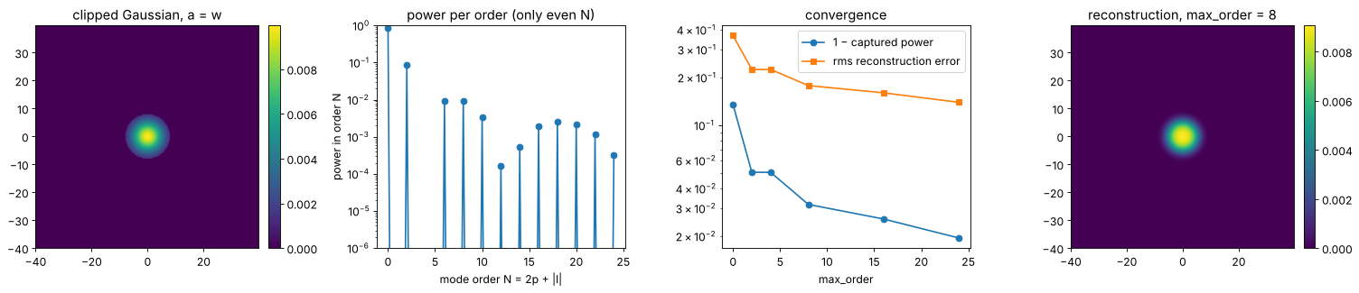
The convergence is slow, as for any field with a hard edge: the error falls roughly like a power of the order, not exponentially. The power in LG\(_{00}\) is the overlap of the clipped beam with the original Gaussian: the overlap integral is the transmitted power \(1 - e^{-2}\), and normalized by that power, the fraction in LG\(_{00}\) is again \(1 - e^{-2}\).

The basis waist matters

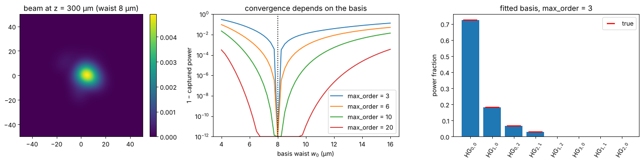
Any \(w_0\) gives a complete basis, but a basis that is too narrow or too wide needs many more modes to describe the same beam. Below, a beam that consists of a few modes of waist 8 µm, observed 300 µm behind its waist, is decomposed in bases with different \(w_0\) (and the correct \(z\)). With w0=None, fit_basis() finds the basis that captures the most power with the given max_order, starting from the second moments and the phase curvature of the field.

# a larger window: wide bases with many modes must fit on the grid
xb, yb, _, _ = grid2d(-100, 100, -100, 100, 320)
z = 300.0
coeffs = {(0, 0): 1.0, (1, 0): 0.5j, (0, 2): 0.3, (2, 1): 0.2*np.exp(1j)}
beam = sum(c*modes.hg_mode(*key, xb, yb, 8.0, wl, z) for key, c in coeffs.items())

w0_values = np.linspace(4, 16, 49)
fig, axes = plt.subplots(1, 3, figsize=(17, 4.2))
show(axes[0], np.abs(beam)**2, "beam at z = 300 µm (waist 8 µm)", [xb[0], xb[-1], yb[0], yb[-1]])
axes[0].set_xlim(-50, 50); axes[0].set_ylim(-50, 50)
for N in (3, 6, 10, 20):
    lost = [1 - modes.decompose_hg(beam, xb, yb, w0_b, wl, z, max_order=N).captured_power for w0_b in w0_values]
    axes[1].semilogy(w0_values, np.maximum(lost, 1E-12), label=f"max_order = {N}")
axes[1].set_ylim(1E-12, 1)
axes[1].axvline(8.0, color="k", ls=":")
axes[1].set_xlabel("basis waist $w_0$ (µm)"); axes[1].set_ylabel("1 − captured power"); axes[1].legend()
axes[1].set_title("convergence depends on the basis")

fit = modes.decompose_hg(beam, xb, yb, wavelength=wl, max_order=3)
print("fitted basis: w0 = {:.4f} µm, z = {:.3f} µm (true 8, 300); captured power {:.1e} short of 1".format(
      fit.basis.w0, fit.basis.z, abs(1 - fit.captured_power)))
bars(axes[2], fit, 8, "fitted basis, max_order = 3")
for i, (key, f) in enumerate(sorted(fit.power_fractions.items(), key=lambda kv: -kv[1])[:4]):
    axes[2].plot(i, abs(coeffs[key])**2/sum(abs(c)**2 for c in coeffs.values()), "r_", ms=25, mew=2)
axes[2].plot([], [], "r_", ms=15, mew=2, label="true"); axes[2].legend()
plt.tight_layout()

fitted basis: w0 = 8.0000 µm, z = 300.000 µm (true 8, 300); captured power 1.6e-15 short of 1

2. A spiral phase plate

A spiral phase plate imprints \(e^{i\varphi}\) on a Gaussian beam. The result has a phase singularity but no dark core yet: it is not the donut mode LG\(_{01}\). Only modes with \(l = 1\) occur, and with the basis waist equal to the beam radius, the projection onto LG\(_{p1}\) can be done analytically (with \(t = 2r^2/w^2\) and \(\int_0^\infty t^{1/2} L_p^1(t) e^{-t} dt = \Gamma(3/2)\Gamma(p + 1/2)/(p!\,\Gamma(1/2)) = \Gamma(p + 1/2)/(2\,p!)\)):

\[ |c_p|^2 = \frac{\Gamma(p + 1/2)^2}{4\,(p!)^2\,(p + 1)}, \qquad |c_0|^2 = \frac{\pi}{4}. \]

Only 78.5 % of the power ends up in the donut mode. The rest goes into radial modes \(p \ge 1\), which form the faint outer rings after propagation. ModeDecomposition.propagate(dz) gives the expansion in another plane: the coefficients stay the same, only the basis moves.

w = 8.0
spiral = modes.hg_mode(0, 0, x, y, w, wl)*np.exp(1j*np.arctan2(Y, X))
d = modes.decompose_lg(spiral, x, y, w, wl, max_order=25)

p = list(range(13))
analytic = [gamma(n + 0.5)**2/(4*factorial(n)**2*(n + 1)) for n in p]
numeric = [d.power_fractions[(n, 1)] for n in p]

# the expansion propagates by changing the basis only (Gouy phases are in the modes):
xp, yp, _, _ = grid2d(-80, 80, -80, 80, 256)
far = d.propagate(2*pi*w**2/wl).reconstruct(xp, yp)   # two Rayleigh lengths

fig, axes = plt.subplots(1, 4, figsize=(19, 4.2))
show(axes[0], np.abs(spiral)**2, "Gaussian × exp(iφ): intensity", extent)
show_phase(axes[1], spiral, "phase", extent)
show(axes[2], np.abs(far)**2, "after 2 Rayleigh lengths (from the modes)", [xp[0], xp[-1], yp[0], yp[-1]])
axes[2].set_xlim(-60, 60); axes[2].set_ylim(-60, 60)
axes[3].semilogy(p, analytic, "k-", label="analytic")
axes[3].semilogy(p, numeric, "o", label="decompose_lg()")
axes[3].set_xlabel("radial index p of LG$_{p1}$"); axes[3].set_ylabel("power fraction"); axes[3].legend()
plt.tight_layout()
print("LG_01: numeric {:.5f}, analytic pi/4 = {:.5f}".format(numeric[0], pi/4))
print("largest |l| != 1 power: {:.1e}".format(max(f for (pp, l), f in d.power_fractions.items() if l != 1)))

LG_01: numeric 0.78538, analytic pi/4 = 0.78540
largest |l| != 1 power: 9.5e-07

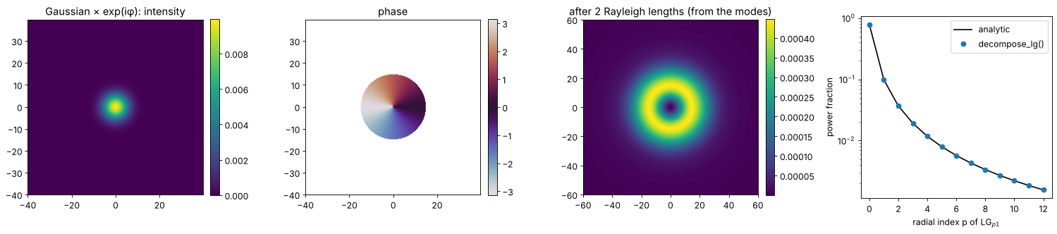
The small deviations at large \(p\) come from sampling the phase singularity at the centre (and from the truncation: the modes beyond max_order hold the last few per cent of the power, because the singular phase decays only slowly in the LG\(_{p1}\) spectrum).

3. M² from the mode content

The Hermite functions are the eigenstates of the quantum harmonic oscillator. With \(\xi = \sqrt{2}x/w_0\), position and direction are \(\xi = (a + a^\dagger)/\sqrt{2}\) and \(p = i(a^\dagger - a)/\sqrt{2}\) in terms of the ladder operators, so the second moments of any coherent superposition follow from sums over the HG coefficients, and

\[ M_x^2 = 2\sqrt{\operatorname{Var}\xi\,\operatorname{Var}p - \operatorname{Cov}(\xi, p)^2}. \]

For a pure mode, \(M_x^2 = 2l + 1\). For a superposition, the cross terms matter: an incoherent mixture of the same modes would give \(\sum_j P_j(2l_j + 1)/P\). ModeDecomposition.M2() evaluates the formula (an LG decomposition is converted to HG first).

First test: a coherent mixture of HG\(_{00}\), HG\(_{10}\), HG\(_{20}\) and HG\(_{02}\) with different phases, a “multimode laser” whose centroid wanders and whose widths change differently from a Gaussian beam along \(z\). The mode content is evaluated in one plane and compared with an ISO 11146 measurement: second moment widths at 21 planes, fitted with beam_quality.fit_caustic().

x2, y2, X2, Y2 = grid2d(-150, 150, -150, 150, 512)
ext2 = [x2[0], x2[-1], y2[0], y2[-1]]
w0 = 10.0
z_R = np.pi*w0**2/wl
c = {(0, 0): 1.0, (1, 0): 0.6j, (2, 0): 0.5*np.exp(0.7j), (0, 2): 0.4}


def laser(z):
    return sum(ci*modes.hg_mode(*key, x2, y2, w0, wl, z) for key, ci in c.items())


d = modes.decompose_hg(laser(0.3*z_R), x2, y2, wavelength=wl, max_order=4)
M2_x, M2_y = d.M2()
P = sum(abs(ci)**2 for ci in c.values())
incoherent_x = sum(abs(ci)**2*(2*l + 1) for (l, m), ci in c.items())/P
print("fitted basis: w0 = {:.4f} µm, z/z_R = {:.4f}".format(d.basis.w0, d.basis.z/z_R))
print("M² from the mode content:  x {:.4f}, y {:.4f}  (incoherent mixture: x {:.4f})".format(M2_x, M2_y, incoherent_x))

zs = np.linspace(-2.5*z_R, 2.5*z_R, 21)
widths = [beam_widths(np.abs(laser(z))**2, x2, y2, iterate=False) for z in zs]
d_x = np.array([wd.d_x if abs(wd.phi) < np.pi/8 else wd.d_y for wd in widths])
d_y = np.array([wd.d_y if abs(wd.phi) < np.pi/8 else wd.d_x for wd in widths])
fits = fit_caustic(zs, d_x, wl), fit_caustic(zs, d_y, wl)
print("M² from the caustic fit:   x {:.4f}, y {:.4f}".format(fits[0].M2, fits[1].M2))

fig, axes = plt.subplots(1, 4, figsize=(20, 4.2))
for ax, z in zip(axes[:3], (-z_R, 0, z_R)):
    show(ax, np.abs(laser(z))**2, f"z = {z/z_R:+.0f} $z_R$", ext2, colorbar=False)
    ax.set_xlim(-50, 50); ax.set_ylim(-50, 50)
zz = np.linspace(zs[0], zs[-1], 200)
for dd, fit, name in ((d_x, fits[0], "x"), (d_y, fits[1], "y")):
    line, = axes[3].plot(zs/z_R, dd/2, "o", label=f"$d_{name}/2$")
    axes[3].plot(zz/z_R, np.sqrt(fit.d_0**2 + fit.theta**2*(zz - fit.z_0)**2)/2, "-", color=line.get_color(),
                 label=f"fit, M² = {fit.M2:.3f}")
axes[3].set_xlabel("z / $z_R$"); axes[3].set_ylabel("radius (µm)"); axes[3].legend(fontsize=9)
axes[3].set_title("ISO 11146 caustic")
plt.tight_layout()

fitted basis: w0 = 10.0000 µm, z/z_R = 0.3000
M² from the mode content:  x 1.7229, y 1.2022  (incoherent mixture: x 1.9718)

M² from the caustic fit:   x 1.7229, y 1.2022

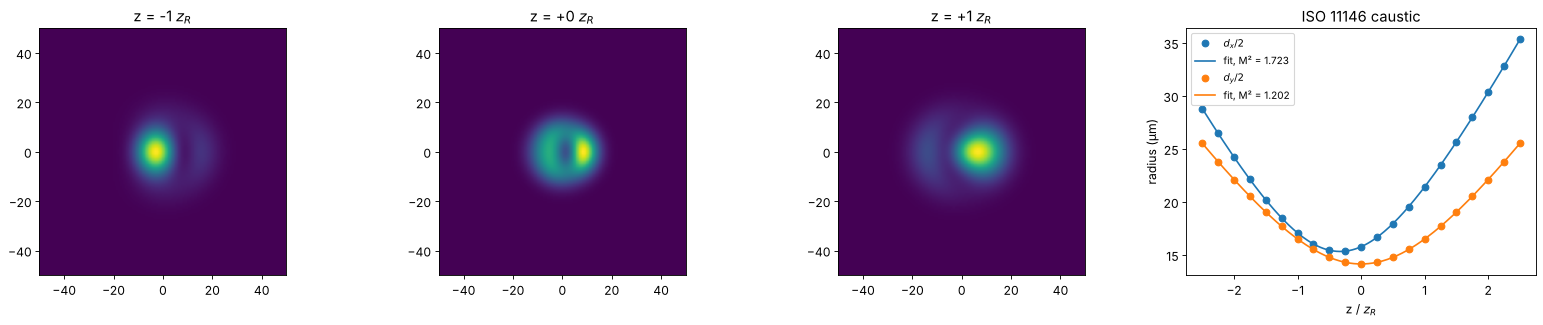
The mode content gives the ISO M² exactly, and different from the incoherent mixture: the phases between modes of the same parity matter.

Truncation and M²

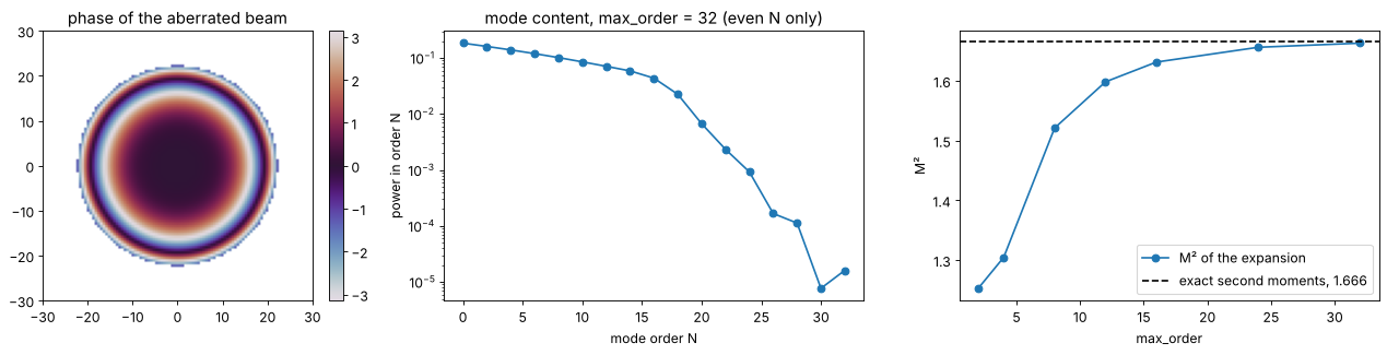
M² is a second moment, and the far wings of the angular spectrum weigh heavily. A Gaussian beam with spherical aberration, phase \(0.3\pi\,(r/w)^4\), has its mode content spread over many orders. With growing max_order, the M² of the expansion converges (from below) to the exact second moment value, here computed from radial integrals of the amplitude \(A\) and the phase gradient, \(\langle\theta_x^2\rangle = \int(|\nabla A|^2 + A^2|\nabla\varphi|^2)/(2k^2P)\). Even when 99.99 % of the power is captured, M² can still be a few per cent low. (The basis is fitted anew for each max_order.)

w = 12.0
alpha = 0.3*np.pi
aberrated = modes.hg_mode(0, 0, x2, y2, w, wl)*np.exp(1j*alpha*((X2**2 + Y2**2)/w**2)**2)

# exact second moments (rotationally symmetric, per axis half of the radial moments):
k = 2*np.pi/wl
A = lambda r: np.exp(-r**2/w**2)
dphi = lambda r: 4*alpha*r**3/w**4
P = quad(lambda r: A(r)**2*r, 0, np.inf)[0]
x2_mean = quad(lambda r: A(r)**2*r**3, 0, np.inf)[0]/(2*P)
th2_mean = quad(lambda r: ((2*r/w**2*A(r))**2 + A(r)**2*dphi(r)**2)*r, 0, np.inf)[0]/(2*P*k**2)
xth_mean = quad(lambda r: A(r)**2*r**2*dphi(r), 0, np.inf)[0]/(2*P*k)
M2_exact = 2*k*np.sqrt(x2_mean*th2_mean - xth_mean**2)

orders = [2, 4, 8, 12, 16, 24, 32]
# a basis fitted for each max_order:
results = [modes.decompose_hg(aberrated, x2, y2, wavelength=wl, max_order=N) for N in orders]

fig, axes = plt.subplots(1, 3, figsize=(17, 4.2))
show_phase(axes[0], aberrated, "phase of the aberrated beam", ext2)
axes[0].set_xlim(-30, 30); axes[0].set_ylim(-30, 30)
axes[1].semilogy(np.arange(0, orders[-1] + 1, 2), results[-1].order_fractions()[::2], "o-")
axes[1].set_xlabel("mode order N"); axes[1].set_ylabel("power in order N")
axes[1].set_title("mode content, max_order = 32 (even N only)")
axes[2].plot(orders, [r.M2()[0] for r in results], "o-", label="M² of the expansion")
axes[2].axhline(M2_exact, color="k", ls="--", label=f"exact second moments, {M2_exact:.3f}")
axes[2].set_xlabel("max_order"); axes[2].set_ylabel("M²"); axes[2].legend()
plt.tight_layout()
for N, r in zip(orders, results):
    print("max_order {:2d}: captured power {:.6f}, M² = {:.4f}".format(N, r.captured_power, r.M2()[0]))

max_order  2: captured power 0.976659, M² = 1.2528
max_order  4: captured power 0.983103, M² = 1.3047
max_order  8: captured power 0.997137, M² = 1.5210
max_order 12: captured power 0.999208, M² = 1.5983
max_order 16: captured power 0.999721, M² = 1.6313
max_order 24: captured power 0.999955, M² = 1.6560
max_order 32: captured power 0.999991, M² = 1.6630

4. LP modes of a step-index fibre

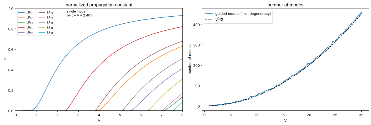
In the weakly guiding approximation (\(n_\mathrm{core} - n_\mathrm{clad} \ll n_\mathrm{core}\), true for telecom fibres with \(\Delta n \approx 0.005\)) the modes are linearly polarized, \(\mathrm{LP}_{lm}\), with

\[\begin{split} E = \begin{cases} J_l(Ur/a)/J_l(U) & r \le a \\ K_l(Wr/a)/K_l(W) & r > a \end{cases} \times \cos(l\varphi) \text{ or } \sin(l\varphi), \qquad U^2 + W^2 = V^2 = \left(\frac{2\pi a}{\lambda}\mathrm{NA}\right)^2, \end{split}\]

and \(U, W\) from the characteristic equation \(U J_{l-1}(U)/J_l(U) = -W K_{l-1}(W)/K_l(W)\) (continuity of the field and its derivative at \(r = a\)). lp_modes(V) finds all guided modes, sorted by the normalized propagation constant \(b = W^2/V^2\), which gives \(n_\mathrm{eff}^2 = n_\mathrm{clad}^2 + b\,(n_\mathrm{core}^2 - n_\mathrm{clad}^2)\). A mode is cut off where \(W \to 0\), at the zeros of \(J_{l-1}\): the fibre is single mode below \(V = 2.405\). Vectorial effects (the splitting of LP modes into HE, EH, TE and TM modes) are not modelled.

V_values = np.linspace(0.3, 8, 300)
curves = {}
for V in V_values:
    for mode in modes.lp_modes(V):
        curves.setdefault((mode.l, mode.m), []).append((V, mode.b))

fig, axes = plt.subplots(1, 2, figsize=(16, 5.5))
for (l, m), points in sorted(curves.items()):
    V_c = modes.lp_cutoff(l, m)
    Vb = np.array([(V_c, 0.0)] + points) if V_c > 0 else np.array(points)
    line, = axes[0].plot(Vb[:, 0], Vb[:, 1], label=f"LP$_{{{l}{m}}}$")
    if V_c > 0:
        axes[0].plot(V_c, 0, "o", color=line.get_color(), ms=4)
axes[0].axvline(2.405, color="k", ls=":", lw=1)
axes[0].text(2.45, 0.92, "single mode\nbelow V = 2.405", fontsize=10)
axes[0].set_xlabel("V"); axes[0].set_ylabel("b"); axes[0].set_ylim(0, 1); axes[0].set_xlim(0, 8)
axes[0].legend(ncol=2, fontsize=9); axes[0].set_title("normalized propagation constant")

V_many = np.linspace(1, 30, 60)
count = [sum(mode.degeneracy for mode in modes.lp_modes(V)) for V in V_many]
axes[1].plot(V_many, count, "o-", ms=3, label="guided modes (incl. degeneracy)")
axes[1].plot(V_many, V_many**2/2, "k--", label="$V^2/2$")
axes[1].set_xlabel("V"); axes[1].set_ylabel("number of modes"); axes[1].legend()
axes[1].set_title("number of modes")
plt.tight_layout()

print("LP01 b(V) against the approximation b = (1.1428 - 0.996/V)**2 (Rudolph and Neumann):")
for V in (1.5, 2.0, 2.405):
    print("  V = {:.3f}: b = {:.4f}, approximation {:.4f}".format(V, modes.lp_mode(0, 1, V).b, (1.1428 - 0.996/V)**2))

LP01 b(V) against the approximation b = (1.1428 - 0.996/V)**2 (Rudolph and Neumann):
  V = 1.500: b = 0.2292, approximation 0.2292
  V = 2.000: b = 0.4162, approximation 0.4158
  V = 2.405: b = 0.5313, approximation 0.5309

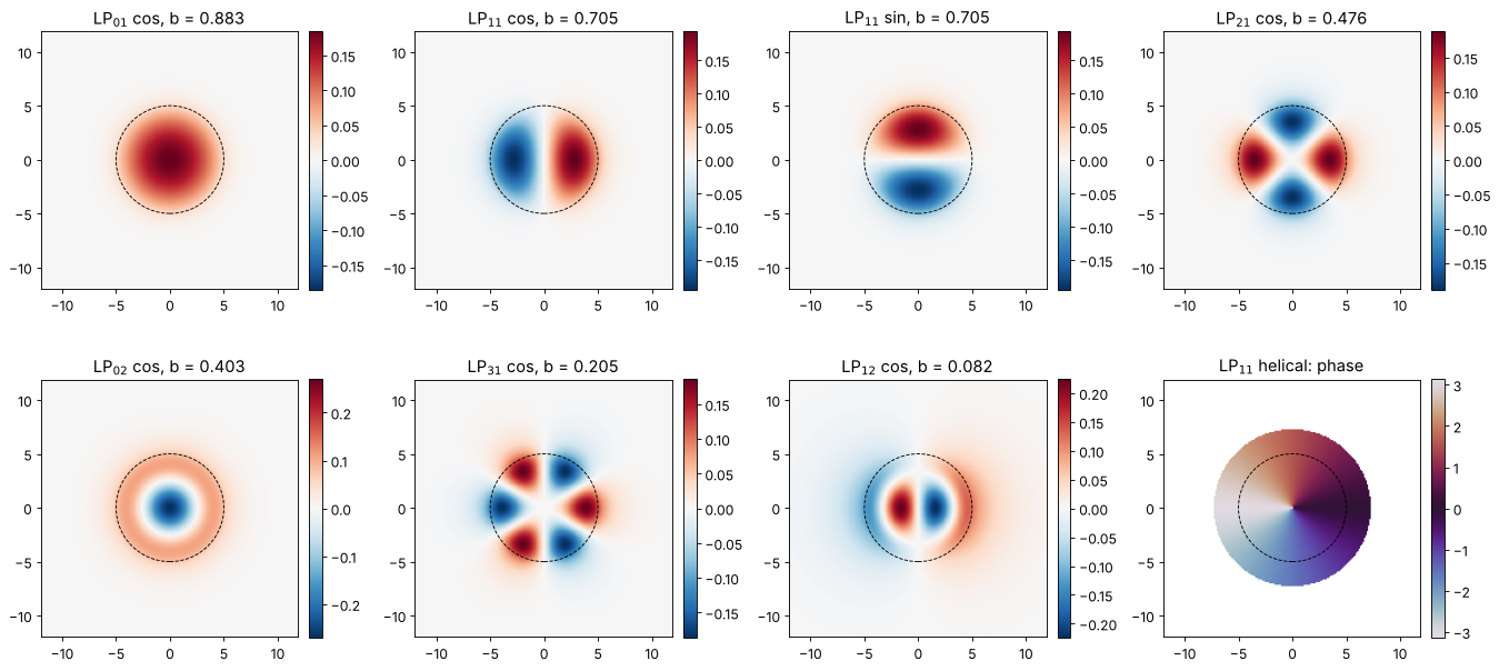
The mode fields of a fibre with \(V = 6\) (core radius 5 µm). Modes with \(l \ge 1\) come in a \(\cos(l\varphi)\) and a \(\sin(l\varphi)\) version (plus two polarizations each); their sum with a phase of 90° is a helical mode \(e^{\pm il\varphi}\) (orientation="+" or "-").

a = 5.0
xf, yf, Xf, Yf = grid2d(-12, 12, -12, 12, 192)
ext_f = [xf[0], xf[-1], yf[0], yf[-1]]
lp = modes.lp_modes(6.0)
fig, axes = plt.subplots(2, 4, figsize=(17, 8))
entries = [(lp[0], "cos"), (lp[1], "cos"), (lp[1], "sin"), (lp[2], "cos"),
           (lp[3], "cos"), (lp[4], "cos"), (lp[5], "cos"), (lp[1], "+")]
for ax, (mode, orientation) in zip(axes.ravel(), entries):
    field = mode.field(xf, yf, a, orientation)
    if orientation == "+":
        show_phase(ax, field, f"LP$_{{{mode.l}{mode.m}}}$ helical: phase", ext_f)
    else:
        lim = np.abs(field).max()
        show(ax, field.real, f"LP$_{{{mode.l}{mode.m}}}$ {orientation}, b = {mode.b:.3f}", ext_f,
             cmap="RdBu_r", vmin=-lim, vmax=lim)
    ax.add_patch(plt.Circle((0, 0), a, fill=False, color="k", ls="--", lw=0.8))
plt.tight_layout()

Marcuse’s Gaussian approximation

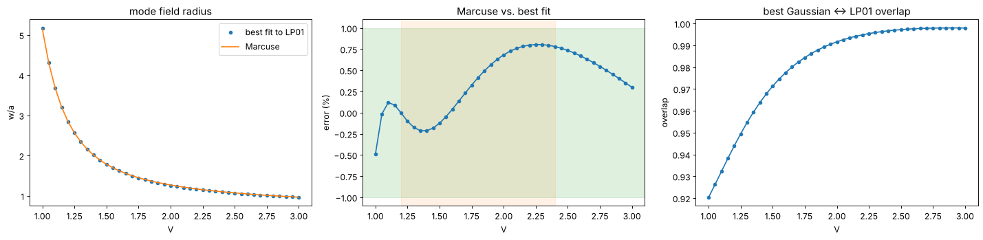
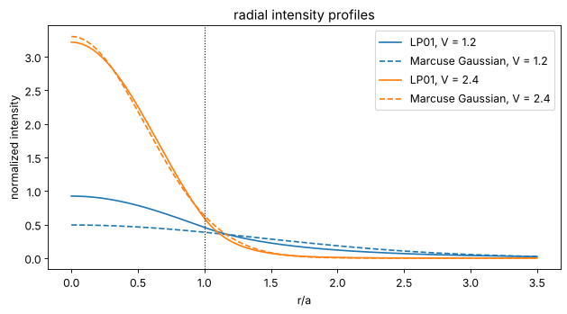
The fundamental mode LP01 looks Gaussian. Marcuse fitted the radius of the best matching Gaussian,

\[ \frac{w}{a} = 0.65 + \frac{1.619}{V^{3/2}} + \frac{2.879}{V^6}, \]

which is accurate to better than 1 % for \(1.2 < V < 2.4\) (marcuse_mode_field_radius(); the mode field diameter is \(2w\)). Below it is compared with the exact best fit (maximum overlap with LP01, from radial integrals). The overlap of the best Gaussian with LP01 exceeds 99 % for \(V > 2\): for single mode fibres, Gaussian beam optics (abcd) is an excellent model. Close to \(V = 1\), LP01 extends far into the cladding with the slowly decaying \(K_0\) tail, and the Gaussian is a poor fit.

def radial_overlap(mode, w, a=1.0):
    f = lambda r: mode.radial(r, a)
    integrate = lambda g: quad(g, 0, a)[0] + quad(g, a, np.inf)[0]
    num = integrate(lambda r: f(r)*np.exp(-r**2/w**2)*r)
    return num**2/(integrate(lambda r: f(r)**2*r)*w**2/4)


V_values = np.linspace(1.0, 3.0, 41)
best_w, best_eta = [], []
for V in V_values:
    mode = modes.lp_mode(0, 1, V)
    res = minimize_scalar(lambda w: -radial_overlap(mode, w), bounds=(0.3, 10), method="bounded",
                          options={"xatol": 1E-10})
    best_w.append(res.x); best_eta.append(-res.fun)
best_w = np.array(best_w)
marcuse = modes.marcuse_mode_field_radius(V_values, 1.0)

fig, axes = plt.subplots(1, 3, figsize=(18, 4.5))
axes[0].plot(V_values, best_w, "o", ms=4, label="best fit to LP01")
axes[0].plot(V_values, marcuse, "-", label="Marcuse")
axes[0].set_xlabel("V"); axes[0].set_ylabel("w/a"); axes[0].legend(); axes[0].set_title("mode field radius")
axes[1].plot(V_values, 100*(marcuse/best_w - 1), "o-", ms=4)
axes[1].axhspan(-1, 1, color="C2", alpha=0.15); axes[1].axvspan(1.2, 2.4, color="C1", alpha=0.1)
axes[1].set_xlabel("V"); axes[1].set_ylabel("error (%)"); axes[1].set_title("Marcuse vs. best fit")
axes[2].plot(V_values, best_eta, "o-", ms=4)
axes[2].set_xlabel("V"); axes[2].set_ylabel("overlap"); axes[2].set_title("best Gaussian ↔ LP01 overlap")
plt.tight_layout()

fig, ax = plt.subplots(figsize=(8, 4.5))
r = np.linspace(0, 3.5, 400)
for V, color in ((1.2, "C0"), (2.4, "C1")):
    mode = modes.lp_mode(0, 1, V)
    w_m = modes.marcuse_mode_field_radius(V, 1.0)
    # scale the Gaussian for maximum overlap (same normalization as the radial overlap):
    norm = quad(lambda s: mode.radial(s, 1)**2*s, 0, np.inf, limit=200)[0]
    ax.plot(r, mode.radial(r, 1)**2/norm, color=color, label=f"LP01, V = {V}")
    ax.plot(r, np.exp(-2*r**2/w_m**2)/(w_m**2/4), "--", color=color, label=f"Marcuse Gaussian, V = {V}")
ax.axvline(1, color="k", ls=":", lw=1)
ax.set_xlabel("r/a"); ax.set_ylabel("normalized intensity"); ax.legend(); ax.set_title("radial intensity profiles")
plt.tight_layout()

5. Coupling into a single mode fibre

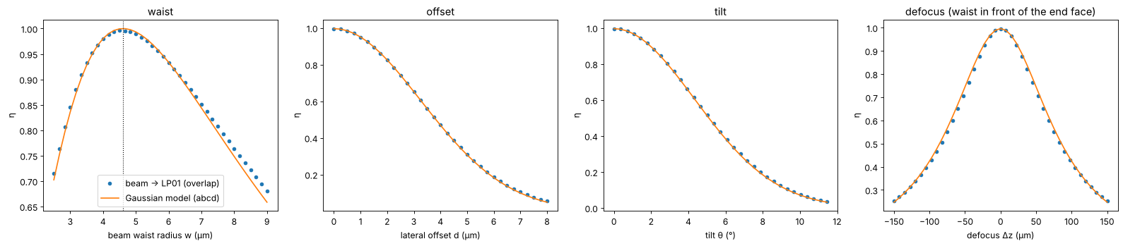
coupling_efficiency(field, mode, x, y) is the normalized overlap \(\eta = |\langle u|E\rangle|^2/(\langle u|u\rangle\langle E|E\rangle)\) of any field with any mode. abcd.coupling_efficiency(q1, q2) gives the same for two Gaussian beams. Here the target is the exact LP01 mode of a fibre similar to SMF-28 at 1550 nm (core radius 4.1 µm, NA 0.14, V = 2.33), and the beam is a Gaussian with radius \(w\) at its waist on the fibre end face.

The Gaussian model (Marcuse radius and the ABCD formula) predicts the curves for the beam waist, a lateral offset \(d\), a tilt \(\theta\) and a defocus \(\Delta z\) very well:

\[ \eta_\mathrm{offset} = \eta_0\,e^{-d^2/w^2}, \qquad \eta_\mathrm{tilt} = \eta_0\,e^{-(\pi n w \theta/\lambda)^2} \qquad (\text{matched } w), \]

but the maximum is \(\eta_0 \approx 99.6\,\%\), not 100 %: LP01 is not exactly Gaussian.

wl_t = 1.55
a, NA, n_clad = 4.1, 0.14, 1.444
n_core = np.sqrt(n_clad**2 + NA**2)
lp01 = modes.lp_modes(core_radius=a, n_core=n_core, n_clad=n_clad, wavelength=wl_t)[0]
V = lp01.V
w_m = modes.marcuse_mode_field_radius(V, a)
print("V = {:.3f}, n_eff = {:.5f}, Marcuse MFD = {:.2f} µm".format(V, lp01.n_eff, 2*w_m))

xs, ys, Xs, Ys = grid2d(-40, 40, -40, 40, 256)
mode = lp01.field(xs, ys, a)
q_fibre = 1j*np.pi*w_m**2/wl_t

fig, axes = plt.subplots(1, 4, figsize=(20, 4.5))
w_values = np.linspace(2.5, 9, 40)
eta_w = [modes.coupling_efficiency(modes.hg_mode(0, 0, xs, ys, w_b, wl_t), mode, xs, ys) for w_b in w_values]
axes[0].plot(w_values, eta_w, "o", ms=4, label="beam → LP01 (overlap)")
axes[0].plot(w_values, [abcd.coupling_efficiency(1j*np.pi*w_b**2/wl_t, q_fibre, wl_t) for w_b in w_values], "-",
             label="Gaussian model (abcd)")
axes[0].axvline(w_m, color="k", ls=":", lw=1)
axes[0].set_xlabel("beam waist radius w (µm)"); axes[0].set_ylabel("η"); axes[0].legend(); axes[0].set_title("waist")

beam = modes.hg_mode(0, 0, xs, ys, w_m, wl_t)
eta0 = modes.coupling_efficiency(beam, mode, xs, ys)
offsets = np.linspace(0, 8, 33)
axes[1].plot(offsets, modes.coupling_vs_offset(beam, mode, xs, ys, offsets), "o", ms=4)
axes[1].plot(offsets, eta0*np.exp(-offsets**2/w_m**2), "-")
axes[1].set_xlabel("lateral offset d (µm)"); axes[1].set_title("offset")

angles = np.linspace(0, 0.2, 33)
axes[2].plot(np.degrees(angles), modes.coupling_vs_tilt(beam, mode, xs, ys, wl_t, angles), "o", ms=4)
axes[2].plot(np.degrees(angles), eta0*np.exp(-(np.pi*w_m*np.sin(angles)/wl_t)**2), "-")
axes[2].set_xlabel("tilt θ (°)"); axes[2].set_title("tilt")

dz = np.linspace(-150, 150, 41)
axes[3].plot(dz, modes.coupling_vs_defocus(beam, mode, xs, ys, wl_t, dz), "o", ms=4)
axes[3].plot(dz, [eta0*abcd.coupling_efficiency(q_fibre + d, q_fibre, wl_t) for d in dz], "-")
axes[3].set_xlabel("defocus Δz (µm)"); axes[3].set_title("defocus (waist in front of the end face)")
for ax in axes[1:]:
    ax.set_ylabel("η")
plt.tight_layout()
print("coupling of a Gaussian with the Marcuse waist into LP01: {:.4f}".format(eta0))

V = 2.327, n_eff = 1.44747, Marcuse MFD = 9.22 µm

coupling of a Gaussian with the Marcuse waist into LP01: 0.9960

Aberrated beams

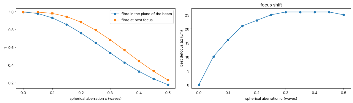
The overlap integral handles any field. A beam focused onto the fibre with spherical aberration, phase \(2\pi\,c\,(6\rho^4 - 6\rho^2 + 1)\) with \(\rho = r/(2w)\), couples worse. Moving the fibre along \(z\) partly compensates the aberration: the best focus shifts, and the loss at best focus is smaller.

rho2 = (Xs**2 + Ys**2)/(2*w_m)**2
coeffs_sa = np.linspace(0, 0.5, 11)
dz_search = np.linspace(-40, 40, 81)
eta_sa, eta_best, dz_best = [], [], []
for c in coeffs_sa:
    field = beam*np.exp(2j*np.pi*c*(6*rho2**2 - 6*rho2 + 1))
    eta_sa.append(modes.coupling_efficiency(field, mode, xs, ys))
    sweep = modes.coupling_vs_defocus(field, mode, xs, ys, wl_t, dz_search)
    eta_best.append(sweep.max()); dz_best.append(dz_search[sweep.argmax()])

fig, axes = plt.subplots(1, 2, figsize=(15, 4.5))
axes[0].plot(coeffs_sa, eta_sa, "o-", label="fibre in the plane of the beam")
axes[0].plot(coeffs_sa, eta_best, "s-", label="fibre at best focus")
axes[0].set_xlabel("spherical aberration c (waves)"); axes[0].set_ylabel("η"); axes[0].legend()
axes[1].plot(coeffs_sa, dz_best, "o-")
axes[1].set_xlabel("spherical aberration c (waves)"); axes[1].set_ylabel("best defocus Δz (µm)")
axes[1].set_title("focus shift")
plt.tight_layout()

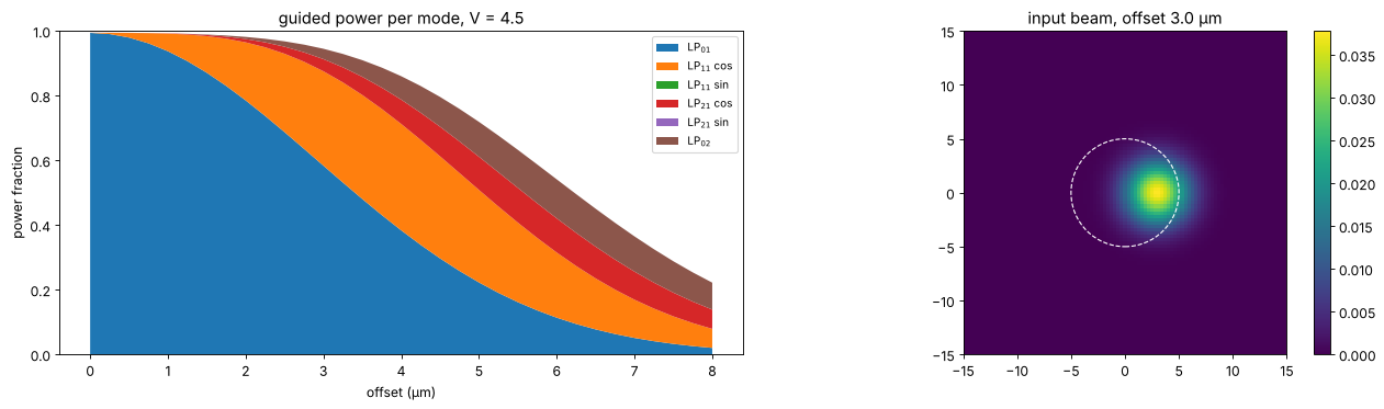
Exciting higher modes in a few-mode fibre

A fibre with \(V = 4.5\) guides LP01, LP11, LP21 and LP02. A Gaussian beam matched to LP01 and shifted along \(x\) excites the odd mode LP11 (cos) first, then LP21 and LP02. mode_power_fractions() gives the power coupled into each mode of a list of (orthogonal) modes; what is missing to 1 is radiated into the cladding. The \(y\)-oriented modes (sin) stay dark because of the mirror symmetry of the shifted beam about the \(x\) axis.

a_fm = 5.0
lp_fm = modes.lp_modes(4.5)
fields, labels = [], []
for m in lp_fm:
    for orientation in (["cos"] if m.l == 0 else ["cos", "sin"]):
        fields.append(m.field(xs, ys, a_fm, orientation))
        labels.append(f"LP$_{{{m.l}{m.m}}}$" + ("" if m.l == 0 else f" {orientation}"))

w_fm = modes.marcuse_mode_field_radius(lp_fm[0].V, a_fm)
shifts = np.linspace(0, 8, 33)
fractions = np.array([modes.mode_power_fractions(modes.hg_mode(0, 0, xs, ys, w_fm, wl, x0=s), fields, xs, ys)
                      for s in shifts])

fig, axes = plt.subplots(1, 2, figsize=(16, 4.8))
axes[0].stackplot(shifts, fractions.T, labels=labels)
axes[0].set_xlabel("offset (µm)"); axes[0].set_ylabel("power fraction"); axes[0].set_ylim(0, 1)
axes[0].legend(loc="upper right", fontsize=9); axes[0].set_title("guided power per mode, V = 4.5")
s_show = 3.0
show(axes[1], np.abs(modes.hg_mode(0, 0, xs, ys, w_fm, wl, x0=s_show))**2, f"input beam, offset {s_show} µm",
     [xs[0], xs[-1], ys[0], ys[-1]])
axes[1].add_patch(plt.Circle((0, 0), a_fm, fill=False, color="w", ls="--"))
axes[1].set_xlim(-15, 15); axes[1].set_ylim(-15, 15)
plt.tight_layout()

Summary

• decompose_hg() and decompose_lg() expand any field in the modes of beams; the modes are normalized on the grid, and fit_basis() picks a waist and curvature that maximize the captured power.

• ModeDecomposition.M2() gives the ISO 11146 M² of the (truncated) expansion, including the coherent cross terms, which an incoherent estimate misses.

• lp_modes() solves the characteristic equation of a weakly guiding step-index fibre; lp_cutoff(), marcuse_mode_field_radius() and lp_mode_field() give cutoffs, the Gaussian approximation and the fields.

• coupling_efficiency() and the sweeps coupling_vs_offset(), coupling_vs_tilt() and coupling_vs_defocus() generalize abcd.coupling_efficiency() to arbitrary fields and modes.

References

• A. E. Siegman, Lasers, University Science Books (1986).

• L. Allen, M. W. Beijersbergen, R. J. C. Spreeuw and J. P. Woerdman, “Orbital angular momentum of light and the transformation of Laguerre-Gaussian laser modes”, Phys. Rev. A 45, 8185-8189 (1992).

• D. Gloge, “Weakly guiding fibers”, Appl. Opt. 10, 2252-2258 (1971).

• A. W. Snyder and J. D. Love, Optical Waveguide Theory, Chapman and Hall (1983).

• D. Marcuse, “Loss analysis of single-mode fiber splices”, Bell Syst. Tech. J. 56, 703-718 (1977).

• B. E. A. Saleh and M. C. Teich, Fundamentals of Photonics, 2nd ed., Wiley (2007).