Gaussian beams, modes and the Gouy phase
The analytic beams in pyoptics.beams (Gauss-Laguerre and Gauss-Hermite) are
exact solutions of the paraxial wave equation. This notebook visualizes them and
compares them with numerical propagation (pyoptics.propagators). The highlight
is the Gouy phase, which can be seen directly in rotating mode superpositions.
Convention: \(\exp(i(kz - \omega t))\). A beam travelling in \(+z\) carries the phase \(e^{+ikz}\), behind the waist the wavefront is diverging (\(R(z) > 0\)), and the Gouy phase enters as \(e^{-i(N+1)\arctan(z/z_R)}\), with the mode order \(N = 2p + |l|\) (LG) or \(N = l + m\) (HG).
Lengths in µm.
import numpy as np
import matplotlib.pyplot as plt
from matplotlib.colors import hsv_to_rgb

from pyoptics import propagators as prop
from pyoptics.beams import gauss_laguerre, gauss_hermite
from pyoptics.masks import thin_lens
from pyoptics.utils import grid1d, grid2d, wavenumber

plt.rcParams.update({"figure.dpi": 100, "image.origin": "lower", "font.size": 11})

wl = 0.5
k = wavenumber(wl)

def complex_to_rgb(U, gamma=0.7):
    """Hue = phase, brightness = amplitude."""
    A = np.abs(U)/np.abs(U).max()
    H = (np.angle(U) + np.pi)/(2*np.pi)
    return hsv_to_rgb(np.dstack([H, np.ones_like(H), A**gamma]))
1. The fundamental mode: beam radius, radius of curvature, Gouy phase
A Gaussian beam with waist radius \(w_0\) has the Rayleigh length \(z_R = \pi w_0^2/\lambda\) and
With a small waist (\(w_0 = 2\lambda\)), wavefronts and beam shape fit into one picture. Shown is the real part of the field (including the carrier \(e^{ikz}\)), i.e. a snapshot of the wave.
w0 = 1.0
z_R = np.pi*w0**2/wl
x = np.linspace(-6, 6, 401)
y0 = np.array([0.0])
z_vals = np.linspace(-3*z_R, 3*z_R, 1201)
field_xz = np.array([gauss_laguerre(0, 0, x, y0, z, w0, z_R, wl)[0] for z in z_vals])

fig, axes = plt.subplots(1, 2, figsize=(13, 4.5), gridspec_kw={"width_ratios": [2.2, 1]})
ext = (z_vals[0], z_vals[-1], x[0], x[-1])
axes[0].imshow(np.real(field_xz).T, extent=ext, aspect="auto", cmap="RdBu_r", interpolation="bilinear")
wz = w0*np.sqrt(1 + (z_vals/z_R)**2)
axes[0].plot(z_vals, wz, "k--", lw=1); axes[0].plot(z_vals, -wz, "k--", lw=1, label="$\\pm w(z)$")
axes[0].plot(z_vals, z_vals*wl/(np.pi*w0), "k:", lw=0.8); axes[0].plot(z_vals, -z_vals*wl/(np.pi*w0), "k:", lw=0.8)
for zz in (-z_R, z_R):
    axes[0].axvline(zz, color="0.4", lw=0.6)
axes[0].set_xlabel("$z$ [µm]"); axes[0].set_ylabel("$x$ [µm]")
axes[0].set_title(f"Re $U(x, z)$, $w_0$ = {w0} µm, $z_R$ = {z_R:.1f} µm (grey lines: $\\pm z_R$)")
axes[0].legend(loc="upper right", fontsize=9)

zz = np.linspace(-5*z_R, 5*z_R, 500)
axes[1].plot(zz/z_R, w0*np.sqrt(1 + (zz/z_R)**2)/w0, label="$w(z)/w_0$")
with np.errstate(divide="ignore"):
    axes[1].plot(zz/z_R, z_R/(zz*(1 + (z_R/zz)**2)), label="$z_R / R(z)$")
axes[1].plot(zz/z_R, np.arctan(zz/z_R)/(np.pi/2), label="$\\psi(z) / (\\pi/2)$")
axes[1].axhline(0, color="0.7", lw=0.5)
axes[1].set_xlabel("$z / z_R$"); axes[1].legend(fontsize=9); axes[1].set_ylim(-1.2, 3)
axes[1].set_title("Beam parameters")
fig.tight_layout()
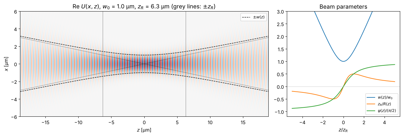
One sees the flat wavefront at the waist, the maximum curvature at \(z = \pm z_R\) and the spherical waves in the far field (dotted: divergence angle \(\theta = \lambda/(\pi w_0)\)). Counting the wave crests on the axis, half a wavelength is missing between \(-\infty\) and \(+\infty\): that is the Gouy phase \(\pi\).
2. Analytic vs. numerical propagation
We take the field at the waist, propagate it with the exact Rayleigh-Sommerfeld
propagator and compare with gauss_laguerre() at \(z\). For \(w_0 = 10\lambda\) the
beam is well paraxial and both agree, including the phase.
w0 = 5.0
z_R = np.pi*w0**2/wl
L, N = 160.0, 512
x, y, X, Y = grid2d(-L/2, L/2, -L/2, L/2, N)
U0 = gauss_laguerre(0, 0, x, y, 0.0, w0, z_R, wl)

fig, axes = plt.subplots(1, 3, figsize=(13, 3.6))
for z, c in zip((0.5*z_R, z_R, 3*z_R), ("C0", "C1", "C2")):
    U_num, _, _ = prop.propagate_padded(prop.rayleigh_sommerfeld_I_TF, U0, x, y, z, wl)
    U_ana = gauss_laguerre(0, 0, x, y, z, w0, z_R, wl)
    lab = f"$z$ = {z/z_R:.1f} $z_R$"
    axes[0].plot(x, np.abs(U_num[N//2])**2, c, lw=2.5, alpha=0.5)
    axes[0].plot(x, np.abs(U_ana[N//2])**2, "k--", lw=0.8)
    sel = np.abs(x) < 2.5*w0*np.sqrt(1 + (z/z_R)**2)
    for U, style in ((U_num, dict(color=c, lw=2.5, alpha=0.5, label=lab)), (U_ana, dict(color="k", ls="--", lw=0.8))):
        ph = np.angle(U[N//2]*np.exp(-1j*k*z))
        # unwrap starting from the centre so that the on-axis value stays in (-pi, pi]:
        ph_unwrapped = np.unwrap(ph[sel])
        ph_unwrapped -= ph_unwrapped[len(ph_unwrapped)//2] - ph[N//2]
        axes[1].plot(x[sel], ph_unwrapped, **style)
    axes[2].semilogy(x, np.abs(U_num[N//2] - U_ana[N//2])/np.abs(U_ana).max(), c, label=lab)
axes[0].set_xlim(-40, 40); axes[0].set_title("Intensity (colour: numerical, --: analytic)", fontsize=10)
axes[1].set_title("Phase without carrier $e^{ikz}$ [rad]", fontsize=10); axes[1].legend(fontsize=8)
axes[2].set_title("relative error $|U_{num} - U_{ana}| / \\max|U|$", fontsize=10); axes[2].set_ylim(1e-8, 1)
for ax in axes:
    ax.set_xlabel("$x$ [µm]")
fig.tight_layout()
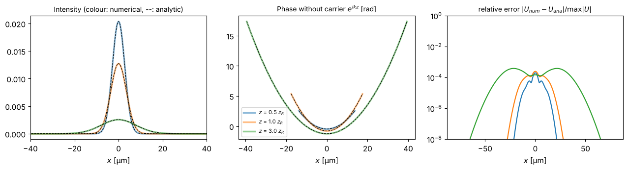
The phase is an upward-opening parabola (\(+k r^2/2R\) with \(R>0\), diverging) on a pedestal: the on-axis value is \(-\psi(z)\), the Gouy phase (\(-\pi/4\) at \(z = z_R\)).
3. The Gouy phase of higher modes, measured numerically
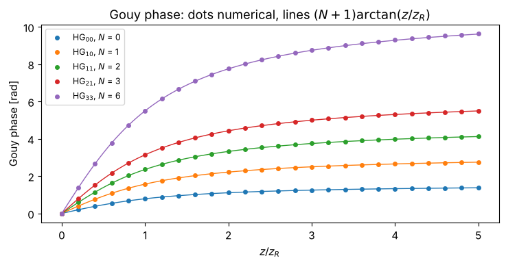
A mode of order \(N\) picks up the Gouy phase \((N+1)\arctan(z/z_R)\). We propagate HG modes numerically and measure the phase relative to the plane wave by projecting the propagated field onto the analytic mode at \(z\) (without Gouy phase).
z_scan = np.linspace(0, 5*z_R, 26)
fig, ax = plt.subplots(figsize=(7.5, 4))
for (l, m), c in zip(((0, 0), (1, 0), (1, 1), (2, 1), (3, 3)), ("C0", "C1", "C2", "C3", "C4")):
    U0 = gauss_hermite(l, m, x, y, 0.0, w0, z_R, wl)
    gouy = []
    for z in z_scan:
        U_num, _, _ = prop.propagate_padded(prop.rayleigh_sommerfeld_I_TF, U0, x, y, z, wl)
        Nmode = l + m
        # analytic mode at z, with the Gouy phase taken out:
        ref = gauss_hermite(l, m, x, y, z, w0, z_R, wl)*np.exp(1j*(Nmode + 1)*np.arctan(z/z_R))*np.exp(-1j*k*z)
        overlap = np.sum(np.conj(ref)*U_num*np.exp(-1j*k*z))
        gouy.append(-np.angle(overlap))
    gouy = np.unwrap(gouy)
    zz = np.linspace(0, 5*z_R, 200)
    ax.plot(zz/z_R, (l + m + 1)*np.arctan(zz/z_R), c, lw=1)
    ax.plot(z_scan/z_R, gouy, "o", color=c, ms=4, label=f"HG$_{{{l}{m}}}$, $N$ = {l+m}")
ax.set_xlabel("$z / z_R$"); ax.set_ylabel("Gouy phase [rad]")
ax.set_title("Gouy phase: dots numerical, lines $(N+1)\\arctan(z/z_R)$")
ax.legend(fontsize=9)
fig.tight_layout()
4. Mode gallery
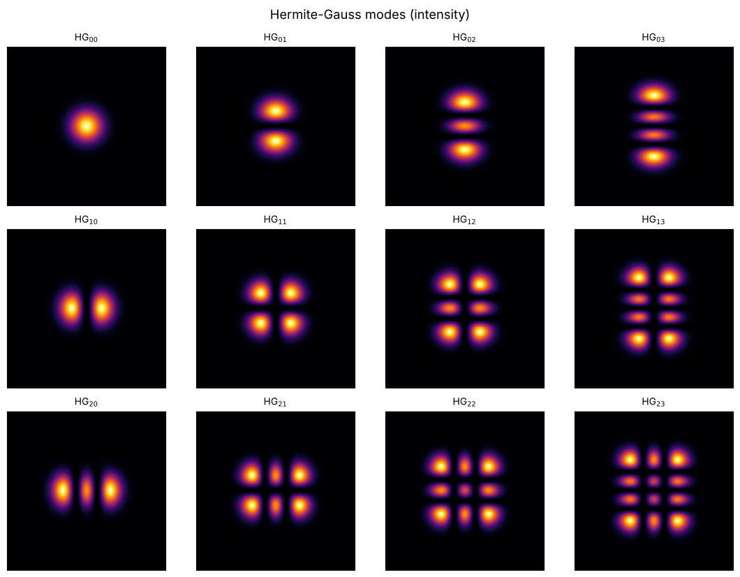
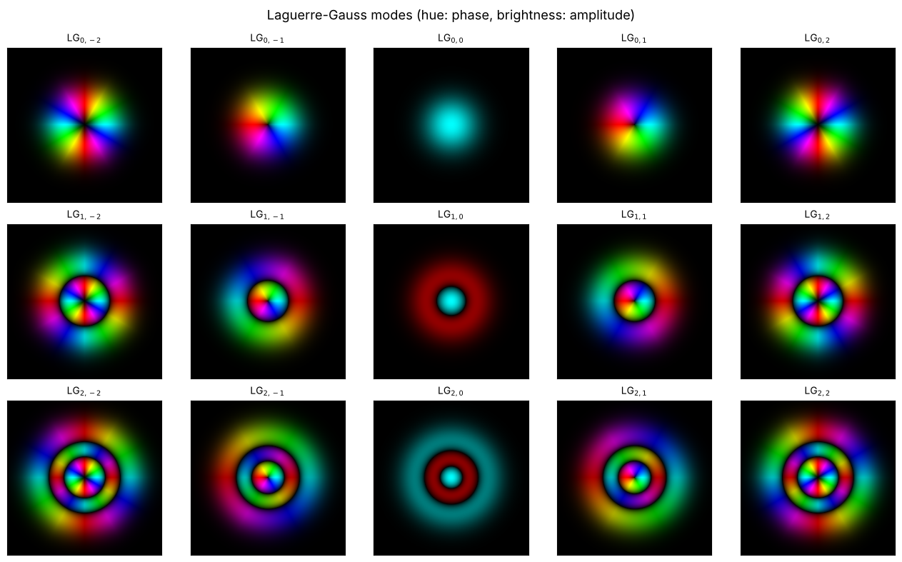
Hermite-Gauss modes HG\(_{lm}\) have \(l\) zeros in \(x\) and \(m\) in \(y\); Laguerre-Gauss modes LG\(_{pl}\) have \(p\) dark rings and a helical phase \(e^{il\varphi}\). For \(l > 0\), every photon carries the orbital angular momentum \(+l\hbar\). In the LG images, hue encodes the phase and brightness the amplitude: for \(l = \pm 1\) the colour wheel goes around the beam axis once, for \(l = \pm 2\) twice, with the opposite sense of rotation for negative \(l\).
Lg, Ng = 30.0, 256
xg, yg, _, _ = grid2d(-Lg/2, Lg/2, -Lg/2, Lg/2, Ng)
w0g = 4.0
z_Rg = np.pi*w0g**2/wl

fig, axes = plt.subplots(3, 4, figsize=(11, 8.4))
for l in range(3):
    for m in range(4):
        U = gauss_hermite(l, m, xg, yg, 0.0, w0g, z_Rg, wl)
        axes[l, m].imshow(np.abs(U)**2, extent=(xg[0], xg[-1], yg[0], yg[-1]), cmap="inferno")
        axes[l, m].set_title(f"HG$_{{{l}{m}}}$", fontsize=10)
        axes[l, m].set_xticks([]); axes[l, m].set_yticks([])
fig.suptitle("Hermite-Gauss modes (intensity)")
fig.tight_layout()
fig, axes = plt.subplots(3, 5, figsize=(13, 8))
for p in range(3):
    for j, l in enumerate(range(-2, 3)):
        U = gauss_laguerre(p, l, xg, yg, 0.0, w0g, z_Rg, wl)
        axes[p, j].imshow(complex_to_rgb(U), extent=(xg[0], xg[-1], yg[0], yg[-1]))
        axes[p, j].set_title(f"LG$_{{{p},{l}}}$", fontsize=10)
        axes[p, j].set_xticks([]); axes[p, j].set_yticks([])
fig.suptitle("Laguerre-Gauss modes (hue: phase, brightness: amplitude)")
fig.tight_layout()
5. The Gouy phase made visible: rotating beams
A superposition of modes of the same order \(N\) keeps its shape on propagation, because all of them pick up the same Gouy phase. An example: HG\(_{10}\) + \(i\) HG\(_{01}\) gives the doughnut mode LG\(_{0,1}\).
For modes of different order, the relative phase changes with \(z\). The superposition LG\(_{0,1}\) + LG\(_{0,3}\) has the Gouy phases \(2\psi\) and \(4\psi\) and the azimuthal phases \(e^{i\varphi}\) and \(e^{3i\varphi}\). The interference term is \(\propto \cos(2\varphi - 2\psi(z))\): two petals that rotate by the angle \(\psi(z) = \arctan(z/z_R)\). From \(-\infty\) to \(+\infty\) that is \(180°\), half of it within \(\pm z_R\). We propagate numerically; the analytic expression only serves as the starting field.
Lr, Nr = 120.0, 256
xr, yr, _, _ = grid2d(-Lr/2, Lr/2, -Lr/2, Lr/2, Nr)
w0r = 5.0
z_Rr = np.pi*w0r**2/wl
U0 = gauss_laguerre(0, 1, xr, yr, 0.0, w0r, z_Rr, wl) + gauss_laguerre(0, 3, xr, yr, 0.0, w0r, z_Rr, wl)
U_start = gauss_laguerre(0, 1, xr, yr, -3*z_Rr, w0r, z_Rr, wl) + gauss_laguerre(0, 3, xr, yr, -3*z_Rr, w0r, z_Rr, wl)

z_show = np.array([-3, -1, -0.3, 0, 0.3, 1, 3])*z_Rr
fig, axes = plt.subplots(1, len(z_show), figsize=(15, 2.9))
for ax, z in zip(axes, z_show):
    U, _, _ = prop.propagate_padded(prop.rayleigh_sommerfeld_I_TF, U_start, xr, yr, z + 3*z_Rr, wl)
    wz = w0r*np.sqrt(1 + (z/z_Rr)**2)
    ax.imshow(np.abs(U)**2, extent=(xr[0]/wz, xr[-1]/wz, yr[0]/wz, yr[-1]/wz), cmap="inferno")
    ax.set_xlim(-2.2, 2.2); ax.set_ylim(-2.2, 2.2)
    ax.set_title(f"$z$ = {z/z_Rr:+.1f} $z_R$", fontsize=10)
    ax.set_xticks([]); ax.set_yticks([])
fig.suptitle("LG$_{0,1}$ + LG$_{0,3}$, propagated numerically from $z = -3z_R$ (axes scaled with $w(z)$)")
fig.tight_layout()

6. Focusing with a thin lens
masks.thin_lens() returns the paraxial lens transmission \(\exp(-ik r^2/2f)\),
which turns a plane wave into a wave converging at \(z = f\). A collimated Gaussian
beam of radius \(w\) is focused to the waist
We compute this with a cylindrical lens (in \(x\) only) and the 1D helper from notebook 01: two \(y\) rows, transfer function propagator.
y_dummy = grid1d(-1, 1, 2)
def propagate_1d(propagator, u, x, z, wl, **kwargs):
    out, _, _ = propagator(np.tile(u, (2, 1)).astype(complex), x, y_dummy, z, wl, **kwargs)
    return out[0]

w_in, f = 200.0, 5000.0
Ll, Nl = 1600.0, 8192
xl = grid1d(-Ll/2, Ll/2, Nl)
u_lens = np.exp(-xl**2/w_in**2)*thin_lens(xl, np.array([0.0]), f, wl)[0]
w_f = wl*f/(np.pi*w_in)
z_Rf = np.pi*w_f**2/wl
z_vals = f + np.linspace(-4*z_Rf, 4*z_Rf, 241)
U_foc = np.array([propagate_1d(prop.rayleigh_sommerfeld_I_TF, u_lens, xl, z, wl) for z in z_vals])

fig, axes = plt.subplots(1, 2, figsize=(13, 4.2), gridspec_kw={"width_ratios": [2, 1]})
axes[0].imshow(np.abs(U_foc).T**2, extent=((z_vals[0] - f), (z_vals[-1] - f), xl[0], xl[-1]),
               aspect="auto", cmap="inferno", interpolation="bilinear")
dz = z_vals - f
axes[0].plot(dz, w_f*np.sqrt(1 + (dz/z_Rf)**2), "w--", lw=1, label="$\\pm w(z)$ for $w_f = \\lambda f/(\\pi w)$")
axes[0].plot(dz, -w_f*np.sqrt(1 + (dz/z_Rf)**2), "w--", lw=1)
axes[0].set_ylim(-5*w_f, 5*w_f); axes[0].legend(loc="upper right", fontsize=9)
axes[0].set_xlabel("$z - f$ [µm]"); axes[0].set_ylabel("$x$ [µm]")
axes[0].set_title(f"Focus of a cylindrical lens, $f$ = {f/1000:.0f} mm, $w$ = {w_in:.0f} µm")

i_f = np.argmin(np.abs(dz))
I_f = np.abs(U_foc[i_f])**2
axes[1].plot(xl, I_f/I_f.max(), lw=2, label="numerical")
axes[1].plot(xl, np.exp(-2*xl**2/w_f**2), "k--", label="Gaussian with $w_f$")
axes[1].set_xlim(-3*w_f, 3*w_f); axes[1].set_xlabel("$x$ [µm]"); axes[1].legend(fontsize=9)
axes[1].set_title(f"Focal plane: $w_f$ = {w_f:.2f} µm")
fig.tight_layout()
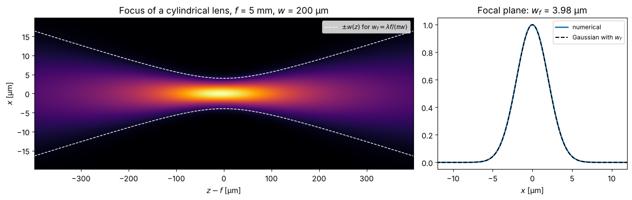
For lenses with a large Fresnel number like this one, the focus lies practically at \(f\). For a small Fresnel number \(N_F = w^2/(\lambda f)\), the intensity maximum moves towards the lens (focal shift). With the tools shown here this is easy to try, e.g. with \(w = 20\) µm and \(f = 5\) mm.
References
A. E. Siegman, Lasers, University Science Books (1986).
H. Kogelnik and T. Li, “Laser beams and resonators”, Appl. Opt. 5, 1550-1567 (1966).
B. E. A. Saleh and M. C. Teich, Fundamentals of Photonics, 2nd ed., Wiley (2007).