Optical proximity correction (OPC)

Near the resolution limit the printed shape of a feature depends on its neighbourhood: isolated lines print at another size than dense ones, line ends pull back, corners round. Optical proximity correction changes the mask so that the printed edges land on the design (the target).

This notebook builds OPC from the pieces of pyoptics.litho, on Manhattan polygons (edges along x and y), with a threshold resist model:

1. Manhattan polygons as masks: MaskLayout.from_polygons() turns any set of rectilinear polygons into an exact union of rectangles, so the diffraction orders stay analytic (no pixelated mask).

2. Rule-based OPC: a bias table through pitch (opc.bias_table()).

3. Forbidden pitches and SRAFs: depth of focus through pitch, and sub-resolution assist features (opc.insert_srafs(), opc.sraf_margin()).

4. Model-based OPC: edges cut into fragments, edge placement errors (EPE) at sites, and the iteration that moves the fragments (opc.FragmentedLayout, opc.edge_placement_errors(), opc.model_opc()): hammerheads, serifs and the corner rounding that remains.

5. Speed: Abbe against the Hopkins TCC and its SOCS kernels.

6. Through focus: OPC is done at one focus and dose.

Setup: ArF water immersion, NA 1.35, 6 % attenuated PSM (thin mask), threshold 0.3 of the open frame; off-axis illumination with TE (azimuthal) polarization for lines, conventional illumination for contacts. The dose is anchored on a simple pattern (lines or a contact array) printing at size.

import time
import numpy as np
import matplotlib.pyplot as plt
from matplotlib.patches import Polygon, Rectangle

from pyoptics.litho import Illumination, LithoSimulation, MaskLayout, Projector, ThinMask
from pyoptics.litho import hopkins, opc

plt.rcParams.update({"figure.dpi": 100, "font.size": 11})

projector = Projector(1.35, 193.0, n=1.437)
stack = ThinMask.att_psm()
THRESHOLD = 0.3


def rect(x0, y0, x1, y1):
    return [(x0, y0), (x1, y0), (x1, y1), (x0, y1)]


def draw(ax, polygons, **kwargs):
    for P in polygons:
        ax.add_patch(Polygon(P, closed=True, **kwargs))


def frame(ax, layout, title):
    ax.set_xlim(-layout.pitch_x/2, layout.pitch_x/2)
    ax.set_ylim(-layout.pitch_y/2, layout.pitch_y/2)
    ax.set_aspect("equal")
    ax.set_title(title)
    ax.set_xlabel("x [nm]")

1. Manhattan polygons as masks

A polygon is a list of vertices; its edges must be parallel to x or y. from_polygons() orients the polygons counterclockwise, merges overlapping ones and cuts the union into non-overlapping rectangles on the grid of all vertex coordinates. The Fourier coefficients of the mask are then sums of products of sinc functions, as for the built-in layouts. The polygons fill one period of a periodic mask; with periods of several \(\lambda/\mathrm{NA}\) the neighbours hardly interact.

Four clips, with 50 nm lines and 80 nm contacts, each in its own period:

clips = {
    "tip to tip": MaskLayout.from_polygons(200, 500, [rect(-25, -215, 25, -35), rect(-25, 35, 25, 215)]),
    "L": MaskLayout.from_polygons(400, 400, [[(-150, -150), (100, -150), (100, -100), (-100, -100),
                                              (-100, 150), (-150, 150)]]),
    "T": MaskLayout.from_polygons(400, 400, [[(-150, -25), (150, -25), (150, 25), (25, 25), (25, 150),
                                              (-25, 150), (-25, 25), (-150, 25)]]),
    "contacts": MaskLayout.from_polygons(400, 400, [rect(-120, -40, -40, 40), rect(40, -100, 120, 100)],
                                         tone="dark"),
}
for name, L in clips.items():
    print("{:10s} {} polygons -> {} rectangles, period {} x {} nm, tone {}".format(
        name, len(L.polygons), len(L.features), L.pitch_x, L.pitch_y, L.tone))

tip to tip 2 polygons -> 2 rectangles, period 200 x 500 nm, tone clear
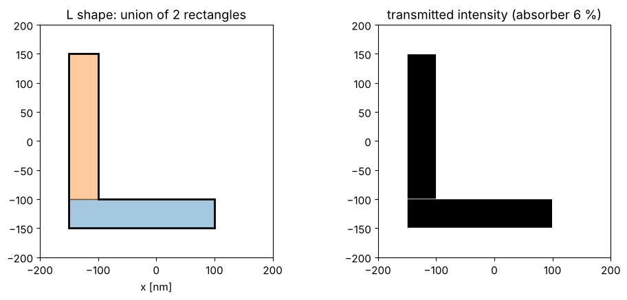
L          1 polygons -> 2 rectangles, period 400 x 400 nm, tone clear
T          1 polygons -> 2 rectangles, period 400 x 400 nm, tone clear
contacts   2 polygons -> 2 rectangles, period 400 x 400 nm, tone dark

The L shape as rectangles, and the transmission sampled from them:

L = clips["L"]
fig, axs = plt.subplots(1, 2, figsize=(10, 4.5))
for k, (x0, y0, a, b) in enumerate(L.features):
    axs[0].add_patch(Rectangle((x0 - a/2, y0 - b/2), a, b, fc="C{}".format(k), alpha=0.4, ec="k"))
draw(axs[0], L.polygons, fill=False, ec="k", lw=2)
frame(axs[0], L, "L shape: union of {} rectangles".format(len(L.features)))
x = np.linspace(-200, 200, 401)
axs[1].imshow(np.abs(L.transmission(x, x, t_absorber=stack.t_absorber))**2, origin="lower",
              extent=(-200, 200, -200, 200), cmap="gray")
axs[1].set_title("transmitted intensity (absorber 6 %)")
plt.tight_layout()

What prints without OPC

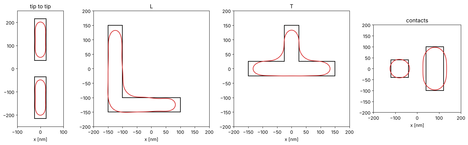
Images of one period on a 2 nm grid (Hopkins, see section 5) and the printed contour at the threshold. The dose prints semi-dense lines (50 nm at 200 nm pitch) at size, for the contacts a square array of 80 nm contacts at 400 nm pitch (with conventional illumination, \(\sigma = 0.5\)). model_opc(max_iter=0) images the uncorrected target and returns the EPEs at the sites (section 4).

annular = Illumination.annular(0.9, 0.6, n_samples=11, polarization="TE")
conventional = Illumination.conventional(0.5, n_samples=11, polarization="unpolarized")
sim_lines = LithoSimulation(MaskLayout.lines_spaces(200, 50), stack, annular, projector)
sim_contacts = LithoSimulation(MaskLayout.contact_holes(400, 80), stack, conventional, projector)
dose_lines = sim_lines.dose_to_size(50, THRESHOLD)
dose_contacts = sim_contacts.dose_to_size(80, THRESHOLD)
print("dose (lines) = {:.3f}, dose (contacts) = {:.3f}".format(dose_lines, dose_contacts))

sims = {name: (sim_contacts if L.tone == "dark" else sim_lines).with_(layout=L) for name, L in clips.items()}
doses = {name: dose_contacts if L.tone == "dark" else dose_lines for name, L in clips.items()}
before = {name: opc.model_opc(sims[name], dose=doses[name], max_iter=0) for name in clips}

fig, axs = plt.subplots(1, 4, figsize=(16, 5), gridspec_kw={"width_ratios": [2, 4, 4, 3]})
for ax, (name, r) in zip(axs, before.items()):
    draw(ax, clips[name].polygons, fill=False, ec="k", lw=1.5)
    ax.contour(r.x, r.y, r.image, [THRESHOLD], colors="C3")
    frame(ax, clips[name], name)
plt.tight_layout()

dose (lines) = 0.799, dose (contacts) = 1.443

r = before["tip to tip"]
ends = r.fragments.sites[:, 0] == 0
print("tip to tip: line end pull back {:.1f} nm (gap {:.0f} nm instead of 70 nm)".format(
    -r.epe[ends].mean(), 70 - 2*r.epe[ends].mean()))
print("(an EPE of 30 nm is the search range: no printed edge within 30 nm of the site)")
for name, r in before.items():
    print("{:10s} max |EPE| = {:5.1f} nm, RMS EPE = {:4.1f} nm".format(name, *r.history[0]))

tip to tip: line end pull back 13.7 nm (gap 97 nm instead of 70 nm)
(an EPE of 30 nm is the search range: no printed edge within 30 nm of the site)
tip to tip max |EPE| =  30.0 nm, RMS EPE = 18.0 nm
L          max |EPE| =  30.0 nm, RMS EPE = 15.1 nm
T          max |EPE| =  30.0 nm, RMS EPE = 17.7 nm
contacts   max |EPE| =  14.9 nm, RMS EPE =  9.2 nm

Line ends pull back (about 14 nm each, the 70 nm gap prints almost 100 nm wide), corners round, the inner corners of the L and the T fill in, the free ends of the L and the T arms shorten. The square contact prints round, the bar contact too wide and a little short. Rules and models fix what can be fixed.

2. Rule-based OPC: bias through pitch

The simplest correction: lines get a mask bias that depends on the space to their neighbours. bias_table() anchors the dose on one pitch (printing at size without bias) and finds, for every pitch, the mask CD that prints the target CD at that dose (root finding on the threshold CD of LithoSimulation.cd()).

For 45 nm lines with a dipole optimized for the dense pitch (100 nm):

dipole = Illumination.dipole(0.9, 0.7, n_samples=15, polarization="TE")
lines = LithoSimulation(MaskLayout.lines_spaces(100, 45), stack, dipole, projector)
pitches = np.arange(100, 501, 20)
t0 = time.time()
bias, dose_dipole = opc.bias_table(lines, pitches, 45.0)
print("bias table: {:.1f} s, dose {:.3f}".format(time.time() - t0, dose_dipole))
cd_nobias = [lines.with_(layout=MaskLayout.lines_spaces(p, 45)).cd(THRESHOLD, dose_dipole) for p in pitches]

fig, axs = plt.subplots(1, 2, figsize=(11, 4))
axs[0].plot(pitches, cd_nobias, "o-", label="no bias")
axs[0].axhline(45, color="k", lw=0.8)
axs[0].set_xlabel("pitch [nm]"), axs[0].set_ylabel("printed CD [nm]")
axs[0].set_title("CD through pitch at one dose"), axs[0].legend()
axs[1].plot(pitches, bias, "o-")
axs[1].set_xlabel("pitch [nm]"), axs[1].set_ylabel("mask bias [nm]")
axs[1].set_title("bias table (mask CD - 45 nm)")
plt.tight_layout()

bias table: 0.4 s, dose 1.099

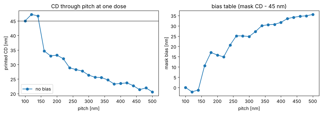
Without bias the isolated lines print much too thin at the dose of the dense ones (with a clear field, more light reaches the line from the open area around it); the table grows to about +35 nm at 500 nm pitch, so the mask line is almost twice as wide as the target. Note the non-monotonic part around 120 to 160 nm pitch: there the bias changes sign, the pitch where the dipole poles stop helping. A real rule deck is such a table (in practice in width and space), applied to every edge pair of the layout; it handles 1D situations but not line ends or corners.

3. Forbidden pitches and SRAFs

The bias puts every pitch on size at best focus, but the depth of focus (DOF: focus range with the CD within ±10 % at the common dose) still depends on the pitch. Off-axis illumination tuned to the dense pitch gives good DOF there and poor DOF at pitches where the diffraction orders fall on the wrong side of the pupil: the forbidden pitches.

foci = np.linspace(-150, 150, 61)


def dof(sim, dose, cd=45.0, tolerance=0.1):
    # contiguous focus range around 0 with the CD in tolerance
    c = sim.fem(foci, [dose], THRESHOLD)[0]
    ok = np.abs(c - cd) <= tolerance*cd
    i = j = len(foci)//2
    if not ok[i]:
        return 0.0
    while i > 0 and ok[i - 1]:
        i -= 1
    while j < len(foci) - 1 and ok[j + 1]:
        j += 1
    return foci[j] - foci[i]


annular_1d = Illumination.annular(0.95, 0.7, n_samples=15, polarization="TE")
results = {}
for name, ill in (("dipole", dipole), ("annular", annular_1d)):
    sim = lines.with_(illumination=ill)
    b, d = opc.bias_table(sim, pitches, 45.0)
    results[name] = (b, d, [dof(sim.with_(layout=MaskLayout.lines_spaces(p, 45 + bb)), d)
                            for p, bb in zip(pitches, b)])

fig, ax = plt.subplots(figsize=(7, 4))
for name, (b, d, D) in results.items():
    ax.plot(pitches, D, "o-", label=name)
ax.set_xlabel("pitch [nm]"), ax.set_ylabel("DOF [nm] (CD ±10 %)")
ax.set_title("DOF through pitch (biased to size)"), ax.legend()
for name, (b, d, D) in results.items():
    print(name, dict(zip(pitches[:6], D[:6])), "... 500 nm:", D[-1])

dipole {np.int64(100): np.float64(240.0), np.int64(120): np.float64(100.0), np.int64(140): np.float64(60.0), np.int64(160): np.float64(90.0), np.int64(180): np.float64(80.0), np.int64(200): np.float64(70.0)} ... 500 nm: 40.0
annular {np.int64(100): np.float64(250.0), np.int64(120): np.float64(120.0), np.int64(140): np.float64(80.0), np.int64(160): np.float64(80.0), np.int64(180): np.float64(80.0), np.int64(200): np.float64(70.0)} ... 500 nm: 50.0

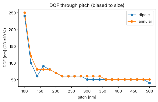
The dipole gives a large DOF at the dense pitch, but drops to a minimum at 140 nm pitch and partly recovers at 160 nm: a forbidden pitch. The annular source does as well at the dense pitch here (45 nm lines at 100 nm pitch are not yet at the limit where only a dipole prints them) and loses DOF smoothly, without the dip. Beyond about 300 nm both are left with the DOF of an isolated line, a few tens of nm.

Sub-resolution assist features (SRAFs, scattering bars) are narrow lines next to a semi-dense or isolated line. They are too narrow to print, but they diffract like the neighbours of a dense pattern, so the main line images (and behaves through focus) more like a dense line. A simple rule: bars of width \(w\) at center distance \(d\) (about the dense pitch) from the line, up to three per side, as long as they keep a space \(w\) to everything; bars from both lines of a space that would collide are merged into one in the middle. insert_srafs() implements this; the bias table is then recomputed with the SRAFs in place (make_layout).

W_SRAF, D_SRAF = 25.0, 100.0


def with_srafs(pitch, cd):
    return opc.insert_srafs(MaskLayout.lines_spaces(pitch, cd), W_SRAF, D_SRAF, count=3)


sim_ann = lines.with_(illumination=annular_1d)
b_sraf, d_sraf = opc.bias_table(sim_ann, pitches, 45.0, make_layout=with_srafs)
D_sraf, margin = [], []
for p, b in zip(pitches, b_sraf):
    s = sim_ann.with_(layout=with_srafs(p, 45 + b))
    D_sraf.append(dof(s, d_sraf))
    margin.append(opc.sraf_margin(s, THRESHOLD, d_sraf, foci=(-75, 0, 75)))
n_sraf = [len(with_srafs(p, 45).features) - 1 for p in pitches]

fig, axs = plt.subplots(1, 2, figsize=(12, 4))
axs[0].plot(pitches, results["annular"][2], "o-", label="annular")
axs[0].plot(pitches, D_sraf, "s-", label="annular + SRAF")
axs[0].set_xlabel("pitch [nm]"), axs[0].set_ylabel("DOF [nm]"), axs[0].legend()
axs[0].set_title("SRAFs {:g} nm at {:g} nm".format(W_SRAF, D_SRAF))
L = with_srafs(400, 45 + b_sraf[list(pitches).index(400)])
x = np.linspace(-400, 400, 801)
for f in (0, 50):
    axs[1].plot(x, d_sraf*sim_ann.with_(layout=L).image(x, focus=f), label="focus {} nm".format(f))
axs[1].plot(x, 0.2*L.transmission(x, t_absorber=0).real + 1.6, "k", lw=1, label="mask")
axs[1].axhline(THRESHOLD, color="k", ls=":")
axs[1].set_xlabel("x [nm]"), axs[1].set_ylabel("dose x intensity"), axs[1].legend(fontsize=9)
axs[1].set_title("pitch 400 nm with {} SRAFs".format(len(L.features) - 1))
plt.tight_layout()
print("SRAFs per period:", {int(p): n for p, n in zip(pitches, n_sraf) if n})
print("SRAF margin (>0: does not print, focus -75..75 nm):",
      {int(p): round(m, 2) for p, m, n in zip(pitches, margin, n_sraf) if n})

SRAFs per period: {160: 1, 180: 1, 200: 1, 220: 1, 240: 1, 260: 2, 280: 2, 300: 2, 320: 2, 340: 2, 360: 3, 380: 3, 400: 3, 420: 3, 440: 3, 460: 4, 480: 4, 500: 4}
SRAF margin (>0: does not print, focus -75..75 nm): {160: 0.01, 180: 0.02, 200: 0.08, 220: 0.27, 240: 0.31, 260: 0.08, 280: 0.2, 300: 0.25, 320: 0.3, 340: 0.35, 360: 0.19, 380: 0.25, 400: 0.28, 420: 0.35, 440: 0.45, 460: 0.23, 480: 0.26, 500: 0.28}

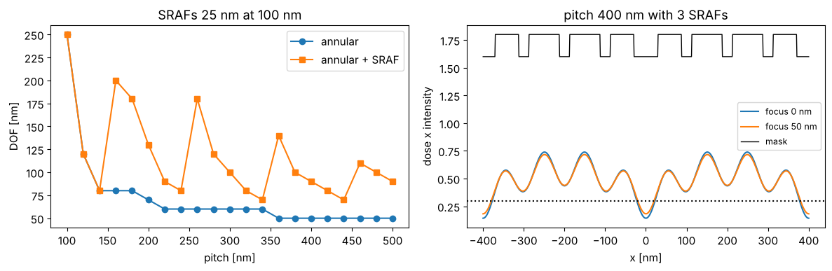
Where they fit (from 160 nm pitch on), the SRAFs lift the DOF of the semi-dense and isolated lines, while the image at their centers stays above the threshold over ±75 nm of focus (sraf_margin() > 0). The margin is smallest (1 to 2 %) at 160 and 180 nm pitch, where one bar sits in the middle of a space of about 120 nm: a real rule deck would leave these pitches without SRAFs or use narrower bars. The DOF through pitch is not smooth: it depends on how many bars fit and where (the rule could be refined per pitch, which is what SRAF rule tables do, or placed by a model). Wider or more closely placed bars help more but start to print; with the attenuated PSM the margin is small because even narrow absorber lines are dark.

4. Model-based OPC

For 2D shapes the correction is computed with the imaging model:

• Fragmentation: every polygon edge is cut into fragments: short ones (corner_length) at the ends of an edge, the rest in pieces of at most max_length. Each fragment can move along its outward normal.

• Sites and EPE: every fragment has a site on the target edge where the edge placement error is measured: the distance from the target edge to the printed contour along the normal (positive: the feature prints too large). The image is computed once per iteration on a grid of one period and interpolated (periodic cubic splines) along the normals.

• Iteration: the moved polygons (with jogs between the fragments of an edge) are imaged again, until the EPEs are small.

F = opc.FragmentedLayout(clips["tip to tip"], max_length=40, corner_length=15)
r = before["tip to tip"]
fig, ax = plt.subplots(figsize=(4, 7))
draw(ax, clips["tip to tip"].polygons, fill=False, ec="k", lw=1)
for k in range(len(F)):
    ax.plot(*np.array([F.start[k], F.end[k]]).T, "-", lw=3, color="C1" if F.corner[k] else "C0")
ax.quiver(*F.sites.T, *(F.normal*r.epe[:, None]).T, angles="xy", scale_units="xy", scale=1,
          color="C3", width=0.01)
ax.contour(r.x, r.y, r.image, [THRESHOLD], colors="C3", linewidths=0.8)
frame(ax, clips["tip to tip"], "{} fragments, EPE arrows".format(len(F)))

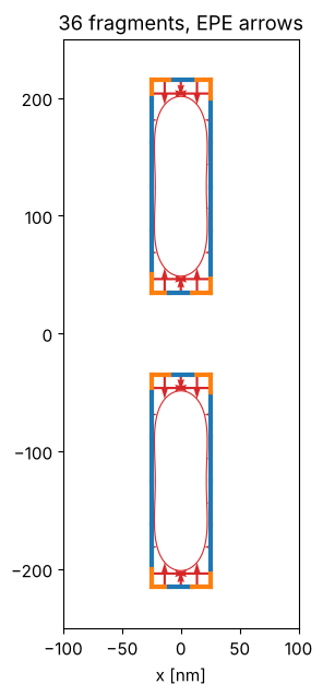
The blue fragments are moved by their EPE, the orange corner fragments measure close to a corner whose printed rounding cannot be removed (their sites sit at 3/4 of the fragment, away from the corner).

Local correction against the Jacobian

The simplest iteration moves every fragment against its own EPE, offset -= damping*EPE (method="local"). But fragments are much shorter than the resolution: moving one changes the EPEs of its neighbours as much as its own, and some combinations (alternating moves of neighbours) change almost nothing. The local scheme then oscillates or produces jagged masks.

method="jacobian" (the default) first measures the response of all EPEs to every fragment move (the Jacobian \(J\), a 2D MEEF matrix, by finite differences of the target: one image per fragment), and then moves all fragments together as the regularized least squares solution

\[\min_{\Delta}\; \lVert W(\mathrm{EPE} + J\Delta)\rVert^2 + \mu \lVert o + \Delta\rVert^2,\]

with \(o\) the current offsets, weights \(W\) (0.3 for the corner sites) and \(\mu\) a small fraction of the mean of \(\mathrm{diag}(J^T W^2 J)\). The regularization keeps the mask close to the target where the EPEs do not care.

sim = sims["tip to tip"]
runs = {m: opc.model_opc(sim, dose=doses["tip to tip"], method=m, max_iter=20) for m in ("local", "jacobian")}

fig, axs = plt.subplots(1, 3, figsize=(13, 6), gridspec_kw={"width_ratios": [2, 2, 3]})
for ax, (m, r) in zip(axs, runs.items()):
    draw(ax, r.layout.polygons, fc="C0", alpha=0.3, ec="C0")
    draw(ax, clips["tip to tip"].polygons, fill=False, ec="k", lw=1)
    ax.contour(r.x, r.y, r.image, [THRESHOLD], colors="C2")
    frame(ax, clips["tip to tip"], m)
for m, r in runs.items():
    axs[2].semilogy(r.history[:, 0], "o-", label=m + ", max")
    axs[2].semilogy(r.history[:, 1], "s--", label=m + ", RMS")
axs[2].set_xlabel("iteration"), axs[2].set_ylabel("|EPE| [nm]"), axs[2].legend()
plt.tight_layout()
for m, r in runs.items():
    edge = ~r.fragments.corner
    print("{:8s}: max |EPE| {:.1f} nm (without corner sites {:.1f} nm), offsets {:.0f} .. {:.0f} nm".format(
        m, r.history[-1, 0], np.abs(r.epe[edge]).max(), r.offsets.min(), r.offsets.max()))

local   : max |EPE| 2.0 nm (without corner sites 2.0 nm), offsets -27 .. 30 nm
jacobian: max |EPE| 6.0 nm (without corner sites 0.6 nm), offsets 1 .. 9 nm

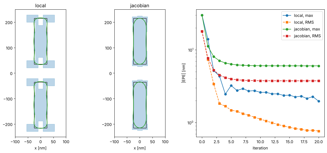
The local scheme reaches small EPEs at all sites, the corner sites included, but only with an extreme mask: the corner fragments run into the offset limit (30 nm), the middle of the line ends is pulled back between them, and the iteration keeps creeping. Such a mask is hard to write and very sensitive to mask errors. The Jacobian solution is smooth and small (offsets of a few nm): a hammerhead at the line ends (the end and its corners are moved out) and a small, even bias along the line. It trades the EPE at the corner sites (6 nm, where the printed contour is round) for a robust mask; the EPEs along the edges are below 1 nm.

All clips

after = {}
t0 = time.time()
for name in clips:
    after[name] = opc.model_opc(sims[name], dose=doses[name])
print("model-based OPC of the 4 clips: {:.1f} s".format(time.time() - t0))

fig, axs = plt.subplots(1, 4, figsize=(16, 5), gridspec_kw={"width_ratios": [2, 4, 4, 3]})
for ax, name in zip(axs, clips):
    draw(ax, after[name].layout.polygons, fc="C0", alpha=0.3, ec="C0")
    draw(ax, clips[name].polygons, fill=False, ec="k", lw=1)
    ax.contour(before[name].x, before[name].y, before[name].image, [THRESHOLD], colors="C3",
               linestyles="--")
    ax.contour(after[name].x, after[name].y, after[name].image, [THRESHOLD], colors="C2")
    frame(ax, clips[name], name)
plt.tight_layout()
print("{:10s} {:>10s} {:>10s} {:>18s}".format("", "max |EPE|", "RMS EPE", "max |EPE| (edges)"))
for name in clips:
    r0, r = before[name], after[name]
    edge = ~r.fragments.corner
    print("{:10s} {:4.1f} -> {:4.1f} {:4.1f} -> {:4.1f} {:12.1f}".format(
        name, r0.history[0, 0], r.history[-1, 0], r0.history[0, 1], r.history[-1, 1], np.abs(r.epe[edge]).max()))

model-based OPC of the 4 clips: 0.9 s
            max |EPE|    RMS EPE  max |EPE| (edges)
tip to tip 30.0 ->  6.0 18.0 ->  3.8          0.6
L          30.0 ->  9.6 15.1 ->  3.7          1.4
T          30.0 -> 10.4 17.7 ->  4.7          1.3
contacts   14.9 -> 10.6  9.2 ->  6.1          2.3

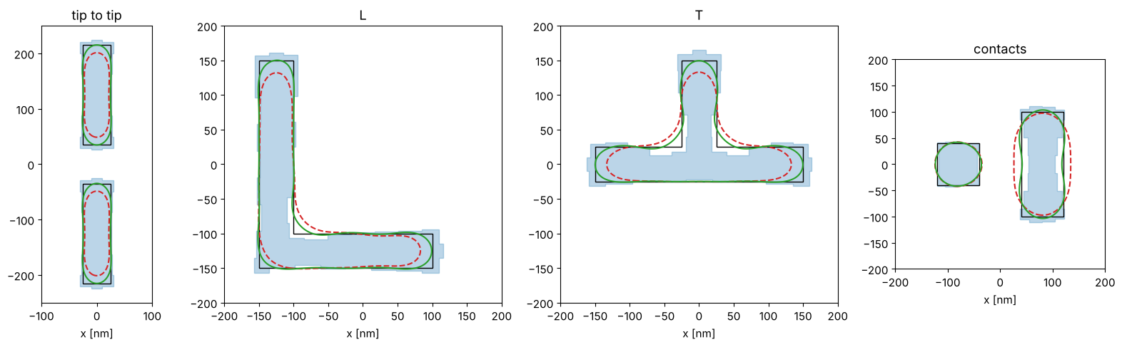
Blue: corrected mask, black: target, red dashed: printed without OPC, green: printed with OPC. The classic shapes appear by themselves: hammerheads at the line ends, serifs on the outer corners, the inner corners of the L and the T cut back, and a “dog bone” for the bar contact (narrowed in the middle, widened at the ends). Along the edges the EPEs are now 1 to 2 nm; the largest remaining errors sit at the corner sites, where the printed contour has a radius of the order of \(0.3\,\lambda/\mathrm{NA}\) that no Manhattan mask removes (the inner corners fill in, the outer corners round off).

5. Speed: Abbe, Hopkins and SOCS

Every iteration needs a 2D image of the moved mask, and the Jacobian needs one per fragment. With Abbe’s method each image is a sum over all source points. The Hopkins TCC of the target is computed once (it depends only on the optics and the pitches) and every mask is then a quadratic form of its spectrum; the SOCS approximation keeps only the leading kernels. For thin masks the Hopkins image is exact.

name = "L"
timing = {}
for imager in ("abbe", "hopkins", "socs"):
    t0 = time.time()
    r = opc.model_opc(sims[name], dose=doses[name], imager=imager)
    timing[imager] = (time.time() - t0, r)
tcc = hopkins.TCC(sims[name])
socs = tcc.socs(energy=0.999)
print("orders: {}, SOCS kernels for 99.9 % of the energy: {}".format(len(tcc.m)*len(tcc.n), socs.n_kernels))
for imager, (t, r) in timing.items():
    print("{:8s} {:5.2f} s, max |EPE| {:.2f} nm, offsets differ from Hopkins by up to {:.2f} nm".format(
        imager, t, r.history[-1, 0], np.abs(r.offsets - timing["hopkins"][1].offsets).max()))

orders: 169, SOCS kernels for 99.9 % of the energy: 78
abbe      0.45 s, max |EPE| 9.64 nm, offsets differ from Hopkins by up to 0.00 nm
hopkins   0.25 s, max |EPE| 9.64 nm, offsets differ from Hopkins by up to 0.00 nm
socs      2.51 s, max |EPE| 9.65 nm, offsets differ from Hopkins by up to 0.07 nm

Hopkins and Abbe give the same correction (the images agree to rounding), SOCS with 99.9 % of the energy differs by a fraction of a nm. Hopkins is the fastest here; its advantage over Abbe grows with the number of source points (the TCC is computed once). SOCS is slower for this clip: 99.9 % of the energy needs 78 kernels for 169 orders, so it does not save anything on a small grid. It pays off for large images with few kernels (a lower energy fraction), which is how full chip OPC uses it.

6. Through focus

The correction is computed at best focus and the nominal dose. Through focus the printed shape changes again: line ends are the most focus sensitive part of a layout.

name = "tip to tip"
r = after[name]
sim_opc = sims[name].with_(layout=r.layout)
fig, axs = plt.subplots(1, 5, figsize=(15, 6))
for ax, f in zip(axs, (-60, -30, 0, 30, 60)):
    I = doses[name]*sim_opc.image(r.x, r.y, focus=f)
    draw(ax, clips[name].polygons, fill=False, ec="k", lw=1)
    ax.contour(r.x, r.y, I, [THRESHOLD], colors="C2")
    y = r.y[np.abs(r.y) < 60]
    cut = doses[name]*sim_opc.image([0.0], y, focus=f)[:, 0]
    gap = np.ptp(y[cut > THRESHOLD]) if np.any(cut > THRESHOLD) else 0.0
    frame(ax, clips[name], "focus {} nm: gap {:.0f} nm".format(f, gap))
plt.tight_layout()

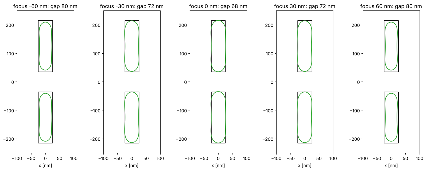
The gap between the line ends (70 nm in the design) is on target at best focus and opens up with defocus, to about 80 nm at 60 nm defocus, while the line width changes much less. Production OPC therefore checks the result over a process window (dose, focus, mask CD) and may trade nominal EPE for robustness; here it is a matter of calling model_opc() with another focus or dose, or checking the corrected mask with LithoSimulation as above.

Summary

• MaskLayout.from_polygons(): Manhattan polygons as exact unions of rectangles, analytic diffraction orders, merging of overlaps.

• Rule-based OPC: bias_table() through pitch at a common dose; SRAFs by rule (insert_srafs()) with a printability check (sraf_margin()); the DOF through pitch shows the forbidden pitch of a dipole and the gain from SRAFs.

• Model-based OPC: FragmentedLayout (fragments, sites, moved polygons), edge_placement_errors() on a periodic image grid and model_opc() with the local or the regularized Jacobian update; Abbe, Hopkins or SOCS imaging.

• Not included: curvilinear masks and inverse lithography, resist models beyond the threshold, mask 3D effects in the 2D layouts (thin masks only), process window OPC, and the flow of a full chip (hierarchy, layout formats).

References

• N. B. Cobb, Fast optical and process proximity correction algorithms for integrated circuit manufacturing, Ph.D. dissertation, University of California, Berkeley (1998).

• A. K.-K. Wong, Resolution Enhancement Techniques in Optical Lithography, SPIE Press (2001).

• R. Socha et al., “Forbidden pitches for 130 nm lithography and below”, Proc. SPIE 4000, 1140 (2000).

• A. K. Wong, R. A. Ferguson and S. M. Mansfield, “The mask error factor in optical lithography”, IEEE Trans. Semicond. Manuf. 13, 235-242 (2000).

• A. Poonawala and P. Milanfar, “Mask design for optical microlithography - an inverse imaging problem”, IEEE Trans. Image Process. 16, 774-788 (2007).

• C. Mack, Fundamental Principles of Optical Lithography: The Science of Microfabrication, Wiley (2007).