Phase unwrapping

Interferometers, holograms, phase shifting algorithms and np.angle() only give the phase modulo \(2\pi\): the wrapped phase \(\psi = \mathcal{W}(\varphi) \in [-\pi, \pi)\). Unwrapping restores \(\varphi = \psi + 2\pi n\) with integers \(n\), assuming that the true phase changes by less than \(\pi\) between neighbouring pixels (the Itoh condition). Then the wrapped differences \(\mathcal{W}(\Delta\psi)\) are the true differences \(\Delta\varphi\), and integrating them gives \(\varphi\) up to a constant.

In 2D the integral may depend on the path: wherever the wrapped differences around a closed loop of \(2\times2\) pixels do not sum to zero there is a residue (a phase vortex, a noise point or an undersampled region). pyoptics.unwrap offers two strategies:

Function	Idea	Result
unwrap_ls(psi)	least squares: the \(\varphi\) whose gradient is closest to \(\mathcal{W}(\nabla\psi)\); a Poisson equation solved by one DCT (Ghiglia and Romero 1994)	smooth, robust, not congruent
unwrap_ls(psi, weights=w, mask=m)	weighted least squares by conjugate gradients, preconditioned with the DCT solver	weights downweight bad pixels
unwrap_ls(..., congruent=True)	the congruent phase nearest to the least squares solution	congruent
unwrap_quality_guided(psi, quality=q)	join pixel pairs in the order of their reliability (Herráez et al. 2002)	congruent, errors confined to bad regions
residues(psi), reliability(psi), wrap(phi), unwrap_1d(psi)	helpers

Congruent means \(\mathcal{W}(\varphi) = \psi\): the result reproduces the data exactly. All functions take arrays indexed [y, x], treat NaN as masked and return NaN outside the mask. The piston is arbitrary; it is chosen such that the result agrees with the data modulo \(2\pi\) and has its mean in \((-\pi, \pi]\).

import time

import numpy as np
import matplotlib.pyplot as plt

from pyoptics.bases import FringeZernikes
from pyoptics.processing import CameraNoiser
from pyoptics.unwrap import (wrap, unwrap_1d, unwrap_ls, unwrap_quality_guided,
                             residues, reliability)
from pyoptics.utils import grid2d

plt.rcParams.update({"figure.dpi": 80, "image.origin": "lower", "font.size": 11})


def show(ax, img, title, cmap="viridis", **kwargs):
    im = ax.imshow(img, extent=extent, cmap=cmap, **kwargs)
    ax.set_title(title)
    ax.set_xticks([]); ax.set_yticks([])
    plt.colorbar(im, ax=ax, fraction=0.046, pad=0.04)
    return im


def remove_piston(u, phi):
    # compare unwrapped results with the truth up to a constant
    d = u - phi
    return d - np.nanmedian(d)


N = 256
x, y, X, Y = grid2d(-1, 1, -1, 1, N)
extent = (x[0], x[-1], y[0], y[-1])

1. One dimension: the Itoh condition

In 1D unwrapping is unique: add \(2\pi\) wherever the wrapped phase jumps by more than \(\pi\) (numpy.unwrap, available as unwrap_1d). It fails as soon as the true phase changes by more than \(\pi\) per sample. Here a quadratic phase (a defocus) gets steeper towards the edge; beyond the sample at which the local phase step reaches \(\pi\), the unwrapped phase falls off the true one.

t = np.linspace(-1, 1, 200)
dt = t[1] - t[0]
fig, axes = plt.subplots(1, 2, figsize=(12, 3.8))
for ax, a in zip(axes, [100, 250]):
    phi = a*t**2
    psi = wrap(phi)
    u = unwrap_1d(psi)
    u += phi[100] - u[100]
    ax.plot(t, phi, "k", lw=3, alpha=0.3, label="true phase")
    ax.plot(t, psi, ".", ms=3, label="wrapped")
    ax.plot(t, u, "C3", label="unwrapped")
    t_lim = np.pi/(2*a*dt)  # |dφ/dt| dt = π
    if t_lim < 1:
        for s in (-1, 1):
            ax.axvline(s*t_lim, color="gray", ls="--")
    ax.set_title(r"$\varphi = %d\,t^2$: max. step %.2f$\pi$" % (a, 2*a*dt/np.pi))
    ax.set_xlabel("t"); ax.set_ylabel("phase (rad)")
axes[0].legend()
plt.tight_layout()

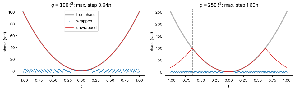
The dashed lines mark where the phase step per sample reaches \(\pi\). Outside of them the samples alias: the unwrapped phase follows a wrong branch. The same limit holds in 2D, where it also produces residues.

2. A wavefront in a circular pupil

A wavefront with defocus, astigmatism, coma and spherical aberration of a few waves each, wrapped many times. Outside the pupil the camera sees noise. Both algorithms recover the wavefront to machine precision once they are told the pupil (mask); without the mask, the noise outside spoils least squares.

Z = FringeZernikes(x, y, R_norm=0.95)
pupil = Z.mask.astype(bool)
phi = Z([4, 5, 7, 9], [30.0, -15.0, 10.0, 8.0])     # radians
rng = np.random.default_rng(1)
psi = np.where(pupil, wrap(phi), rng.uniform(-np.pi, np.pi, phi.shape))

u_ls_nomask = unwrap_ls(psi)
u_ls = unwrap_ls(psi, mask=pupil)
u_qg = unwrap_quality_guided(psi, mask=pupil)

fig, axes = plt.subplots(2, 3, figsize=(14, 8))
show(axes[0, 0], np.where(pupil, phi, np.nan), "true wavefront (rad)")
show(axes[0, 1], psi, "wrapped measurement", cmap="twilight")
show(axes[0, 2], u_qg, "quality guided, with mask")
show(axes[1, 0], np.where(pupil, remove_piston(u_ls_nomask, phi), np.nan),
     "LS without mask: error (rad)", cmap="RdBu_r")
show(axes[1, 1], remove_piston(u_ls, phi), "LS with mask: error (rad)", cmap="RdBu_r")
show(axes[1, 2], remove_piston(u_qg, phi), "quality guided: error (rad)", cmap="RdBu_r")
plt.tight_layout()

for name, u in [("LS, no mask", np.where(pupil, u_ls_nomask, np.nan)),
                ("LS, mask", u_ls), ("quality guided", u_qg)]:
    print("%-16s max |error| = %.2e rad" % (name, np.nanmax(np.abs(remove_piston(u, phi)))))

LS, no mask      max |error| = 6.96e+00 rad
LS, mask         max |error| = 1.15e-09 rad
quality guided   max |error| = 1.42e-14 rad

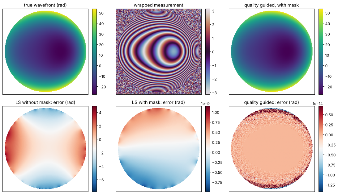
With the mask, the weighted least squares solver needs only a few conjugate gradient iterations, since the unweighted DCT solver is an excellent preconditioner:

_, info = unwrap_ls(psi, mask=pupil, return_info=True)
print(info)

{'iterations': 14, 'residual': np.float64(3.900583437211906e-11)}

3. Residues: where the path matters

A field with an optical vortex pair, \((x - x_1 + i(y - y_1))\,(x - x_2 - i(y - y_2))\), has a phase singularity of charge \(+1\) at \((x_1, y_1)\) and \(-1\) at \((x_2, y_2)\), on top of a smooth wavefront. residues() finds them: the wrapped differences around the \(2\times2\) loop containing a core add up to \(\pm 2\pi\).

No continuous phase can represent this field: any congruent unwrapped phase needs a \(2\pi\) jump (a branch cut) that connects the two vortices.

• Least squares spreads the inconsistency over the whole image: the result is smooth everywhere, but it is not congruent (\(\mathcal{W}(\varphi_{LS}) \neq \psi\)) and is distorted around the vortices.

• congruent=True snaps it to the data; the cut appears where the least squares solution is \(\pi\) away from it.

• The quality guided algorithm puts the cut through the least reliable pixels, which are near the vortices.

x1, y1, x2, y2 = -0.35, 0.1, 0.4, -0.15
smooth = 6*np.exp(-(X**2 + Y**2)/0.5) + 4*X
E = (X - x1 + 1j*(Y - y1))*(X - x2 - 1j*(Y - y2))*np.exp(1j*smooth)
psi_v = np.angle(E)
res = residues(psi_v)
print("residues: %d positive, %d negative, total charge %d"
      % (np.sum(res > 0), np.sum(res < 0), res.sum()))

u_ls = unwrap_ls(psi_v)
u_ls_c = unwrap_ls(psi_v, congruent=True)
u_qg = unwrap_quality_guided(psi_v)

fig, axes = plt.subplots(2, 3, figsize=(14, 8))
show(axes[0, 0], psi_v, "wrapped phase of a vortex pair", cmap="twilight")
iy, ix = np.nonzero(res)
xc, yc = x[:-1] + (x[1] - x[0])/2, y[:-1] + (y[1] - y[0])/2
axes[0, 0].scatter(xc[ix], yc[iy], c=res[iy, ix], cmap="bwr", vmin=-1, vmax=1,
                   s=80, edgecolors="k")
show(axes[0, 1], np.log10(reliability(psi_v)[1:-1, 1:-1]), "log10 reliability")
show(axes[0, 2], wrap(u_ls - psi_v), r"LS: $\mathcal{W}(\varphi_{LS} - \psi)$",
     cmap="RdBu_r", vmin=-np.pi, vmax=np.pi)
show(axes[1, 0], u_ls, "least squares (smooth)")
show(axes[1, 1], u_ls_c, "least squares, congruent")
show(axes[1, 2], u_qg, "quality guided")
for ax in axes[1]:
    ax.plot([x1, x2], [y1, y2], "w.", ms=10)
plt.tight_layout()

residues: 1 positive, 1 negative, total charge 0

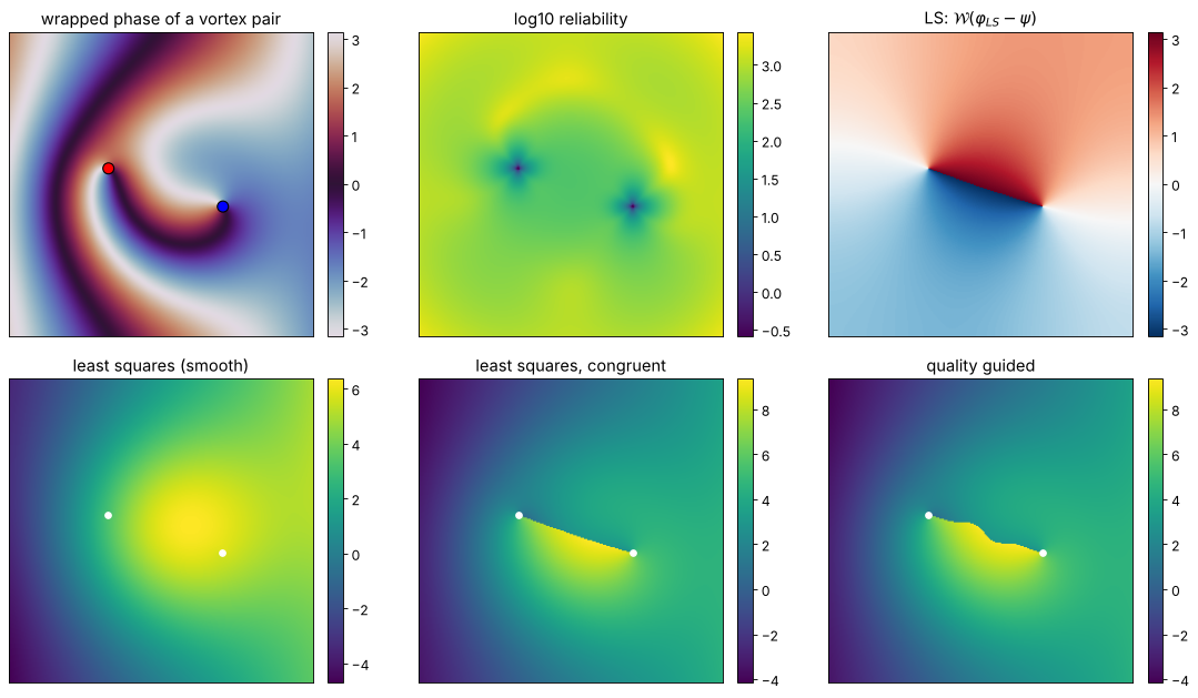
The top right panel shows how far the smooth least squares solution is from the data: up to \(\pi\) along the line between the vortices, and still visibly off elsewhere. The two congruent results both contain a cut that starts and ends on the vortices (white dots), only its route differs.

4. Noise and low modulation

Real wrapped phases are noisy. We take the field \(\sqrt{N_\mathrm{ph}}\,a(x,y)\,e^{i\varphi}\), whose amplitude \(a\) drops to almost zero in two dark spots (e.g. dust particles), add complex Gaussian camera noise with CameraNoiser, and unwrap \(\psi = \arg E\). The phase noise is about \(1/(\sqrt{N_\mathrm{ph}}\,a)\), so the dark spots are pure noise and full of residues.

• Unweighted least squares lets the noise in the spots bend the result around them.

• Weighting by the measured intensity \(|E|^2\) suppresses the spots.

• Quality guided unwrapping with the reliability map (or the amplitude as quality) unwraps the good pixels first.

phi = 25*np.exp(-((X - 0.2)**2 + (Y + 0.1)**2)/0.3) + 8*Y
a = np.exp(-(X**2 + Y**2)/2)  # Gaussian illumination with two dust spots
a *= 1 - 0.98*np.exp(-((X + 0.35)**2 + (Y - 0.2)**2)/0.15**2)
a *= 1 - 0.98*np.exp(-((X - 0.5)**2 + (Y + 0.5)**2)/0.1**2)
noiser = CameraNoiser("gaussian", sigma=1.0, rng=3)
E_n = noiser(np.sqrt(400.0)*a*np.exp(1j*phi))
psi_n = np.angle(E_n)
A = np.abs(E_n)

results = {
    "LS, unweighted": unwrap_ls(psi_n),
    "LS, weights |E|²": unwrap_ls(psi_n, weights=A**2),
    "quality guided (reliability)": unwrap_quality_guided(psi_n),
    "quality guided (|E|)": unwrap_quality_guided(psi_n, quality=A),
}

good = a > 0.3  # where the measurement is meaningful
fig, axes = plt.subplots(2, 3, figsize=(14, 8))
show(axes[0, 0], A, "measured amplitude |E|", cmap="gray")
show(axes[0, 1], psi_n, "wrapped noisy phase", cmap="twilight")
r = residues(psi_n)
show(axes[0, 2], a, "illumination a and residues (%d)" % np.count_nonzero(r), cmap="gray")
iy, ix = np.nonzero(r)
xc, yc = x[:-1] + (x[1] - x[0])/2, y[:-1] + (y[1] - y[0])/2
axes[0, 2].scatter(xc[ix], yc[iy], c=r[iy, ix], cmap="bwr", vmin=-1, vmax=1, s=12)
for ax, (name, u) in zip(axes[1], list(results.items())[:2] + list(results.items())[3:]):
    d = remove_piston(u, phi)
    show(ax, np.where(good, d, np.nan), name + ": error", cmap="RdBu_r", vmin=-1, vmax=1)
plt.tight_layout()

print("rms error where a > 0.3 (expected phase noise %.3f rad):"
      % np.sqrt(np.mean(1/(400*a[good]**2))))
for name, u in results.items():
    d = remove_piston(u, phi)[good]
    d -= np.median(d)
    print("  %-30s %.3f rad, pixels off by 2π: %d"
          % (name, np.sqrt(np.mean(d**2)), np.sum(np.abs(d) > np.pi)))

rms error where a > 0.3 (expected phase noise 0.075 rad):
  LS, unweighted                 0.106 rad, pixels off by 2π: 0
  LS, weights |E|²               0.075 rad, pixels off by 2π: 0
  quality guided (reliability)   0.075 rad, pixels off by 2π: 0
  quality guided (|E|)           0.075 rad, pixels off by 2π: 0

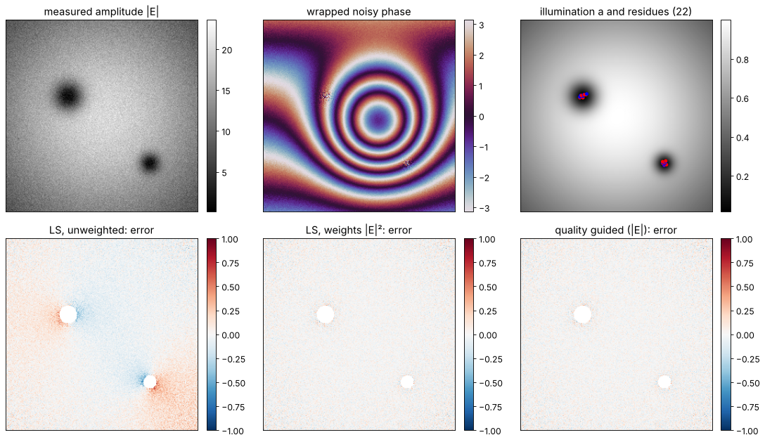
The unweighted least squares solution is smooth but biased around the spots, with errors well above the noise. Weights remove the bias. The quality guided results are congruent, so their error equals the measurement noise on the good pixels.

Error versus signal

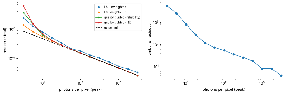
The rms error over the well exposed region as a function of the photon number. At low signal, residues appear everywhere and every method breaks down. From about 100 photons per pixel on, the quality guided and the weighted least squares results reach the noise limit \(1/(\sqrt{N_\mathrm{ph}}\,a)\).

photons = np.logspace(0.5, 3.5, 13)
names = list(results)
err = {n: [] for n in names}
n_res = []
for Nph in photons:
    E_n = CameraNoiser("gaussian", sigma=1.0, rng=5)(np.sqrt(Nph)*a*np.exp(1j*phi))
    psi_n, A = np.angle(E_n), np.abs(E_n)
    n_res.append(np.count_nonzero(residues(psi_n)))
    us = [unwrap_ls(psi_n), unwrap_ls(psi_n, weights=A**2),
          unwrap_quality_guided(psi_n), unwrap_quality_guided(psi_n, quality=A)]
    for n, u in zip(names, us):
        d = remove_piston(u, phi)[good]
        err[n].append(np.sqrt(np.mean((d - np.median(d))**2)))

fig, axes = plt.subplots(1, 2, figsize=(12, 4))
for n in names:
    axes[0].loglog(photons, err[n], "o-", ms=4, label=n)
axes[0].loglog(photons, [np.sqrt(np.mean(1/(p*a[good]**2))) for p in photons],
               "k--", label="noise limit")
axes[0].set_xlabel("photons per pixel (peak)"); axes[0].set_ylabel("rms error (rad)")
axes[0].legend(fontsize=9)
axes[1].loglog(photons, n_res, "o-")
axes[1].set_xlabel("photons per pixel (peak)"); axes[1].set_ylabel("number of residues")
plt.tight_layout()

5. Holes and disconnected regions

Pupils often have holes: a central obscuration, spider vanes, dust. Pass them as mask, or as NaN in the wrapped phase. Regions that are not connected by valid pixels cannot be related to each other, so the quality guided algorithm gives each of them its own piston (a multiple of \(2\pi\)). Least squares connects them only through its smoothness, i.e. by arbitrary, not even \(2\pi\)-quantized offsets.

R = np.hypot(X, Y)
phi = Z([4, 5, 7, 9], [30.0, -15.0, 10.0, 8.0]) + 20*Y
mask = (R < 0.95) & (R > 0.3) & (np.abs(Y) > 0.03)  # obscuration and a spider vane
mask &= np.hypot(X - 0.5, Y - 0.4) > 0.08          # dust
psi = np.where(mask, wrap(phi), np.nan)
u = unwrap_quality_guided(psi)
u_ls = unwrap_ls(psi)

fig, axes = plt.subplots(1, 3, figsize=(14, 4.2))
show(axes[0], psi, "wrapped, NaN outside", cmap="twilight")
show(axes[1], u, "quality guided")
show(axes[2], u - phi, "error: one constant per region", cmap="RdBu_r")
plt.tight_layout()
for region, name in [(Y > 0, "upper half"), (Y < 0, "lower half")]:
    d = (u - phi)[mask & region]
    print("%s: offset %.6f·2π, spread %.1e rad" % (name, np.mean(d)/(2*np.pi), np.ptp(d)))
print("least squares: max. error spread over all regions %.2f rad" % np.nanmax(np.abs(remove_piston(u_ls, phi))))

upper half: offset -2.000000·2π, spread 2.1e-14 rad
lower half: offset 1.000000·2π, spread 1.2e-14 rad
least squares: max. error spread over all regions 1.67 rad

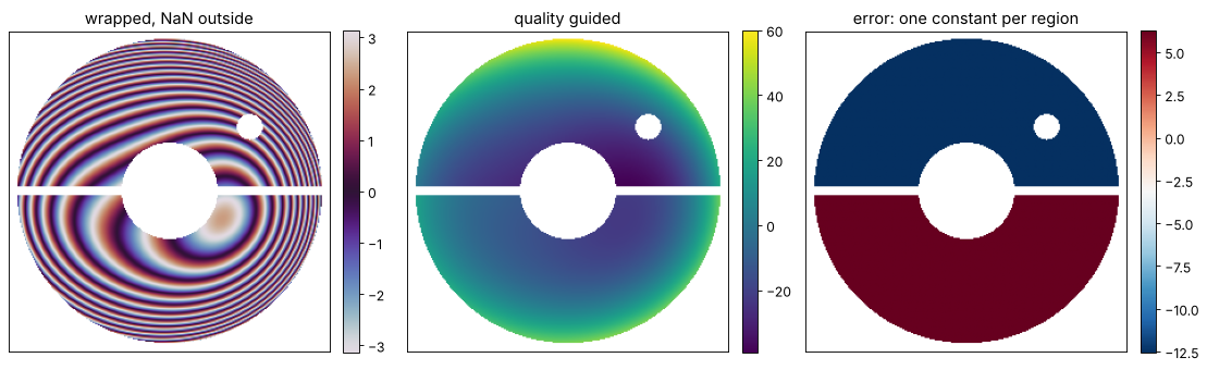
Within each half the error is constant to machine precision, but the two halves are off by different multiples of \(2\pi\). This ambiguity only additional information (another measurement, or a model of the wavefront) can resolve.

6. Speed

The DCT solver is an \(O(N^2 \log N)\) operation. The quality guided algorithm is dominated by sorting the \(2N^2\) edges plus a Python loop over them (union-find), which still unwraps a megapixel image in a few seconds.

for n in [128, 256, 512, 1024]:
    xs, ys, Xs, Ys = grid2d(-1, 1, -1, 1, n)
    psi_s = wrap(40*np.exp(-(Xs**2 + Ys**2)/0.3) + 10*Xs)
    times = []
    for f, kw in [(unwrap_ls, {}), (unwrap_ls, {"weights": np.ones((n, n))}),
                  (unwrap_quality_guided, {})]:
        t0 = time.perf_counter(); f(psi_s, **kw); times.append(time.perf_counter() - t0)
    print("N = %4d: LS (DCT) %.3f s, weighted LS (PCG) %.3f s, quality guided %.2f s"
          % (n, *times))

N =  128: LS (DCT) 0.003 s, weighted LS (PCG) 0.003 s, quality guided 0.05 s

N =  256: LS (DCT) 0.009 s, weighted LS (PCG) 0.018 s, quality guided 0.23 s

N =  512: LS (DCT) 0.061 s, weighted LS (PCG) 0.087 s, quality guided 1.05 s

N = 1024: LS (DCT) 0.521 s, weighted LS (PCG) 0.518 s, quality guided 4.43 s

Summary

• Use unwrap_quality_guided() when the result has to reproduce the data (metrology, phase maps that are compared pixel by pixel). Give it a quality map such as the modulation of a phase shifting measurement if you have one.

• Use unwrap_ls() for a smooth, robust estimate, with weights (modulation, amplitude) and mask whenever parts of the image are bad, and congruent=True to snap it back to the data.

• Check residues() first: without residues all methods agree exactly (up to the piston); many residues mean undersampling or too much noise.

References

• K. Itoh, “Analysis of the phase unwrapping algorithm”, Appl. Opt. 21, 2470 (1982).

• R. M. Goldstein, H. A. Zebker and C. L. Werner, “Satellite radar interferometry: two-dimensional phase unwrapping”, Radio Sci. 23, 713-720 (1988).

• D. C. Ghiglia and L. A. Romero, “Robust two-dimensional weighted and unweighted phase unwrapping that uses fast transforms and iterative methods”, J. Opt. Soc. Am. A 11, 107-117 (1994).

• M. A. Herráez, D. R. Burton, M. J. Lalor and M. A. Gdeisat, “Fast two-dimensional phase-unwrapping algorithm based on sorting by reliability following a noncontinuous path”, Appl. Opt. 41, 7437-7444 (2002).

• D. C. Ghiglia and M. D. Pritt, Two-Dimensional Phase Unwrapping: Theory, Algorithms, and Software, Wiley (1998).