Interfaces and thin films

This notebook covers pyoptics.interfaces (Fresnel coefficients of a single interface) and pyoptics.thin_films (transfer matrix calculation for layer stacks). Topics: Brewster angle, total internal reflection with the evanescent wave, metal reflection, soap film colours, anti-reflection coating, Bragg mirror, thick (incoherent) plates and thin metal films.

Convention: \(\exp(i(\mathbf{k}\cdot\mathbf{r} - \omega t))\); absorbing media have \(\tilde n = n + i\kappa\) with \(\kappa > 0\). The refracted angle is chosen such that the transmitted wave decays away from the interface.

import numpy as np
import matplotlib.pyplot as plt

from pyoptics import interfaces as itf
from pyoptics import thin_films as tf

plt.rcParams.update({"figure.dpi": 100, "image.origin": "lower", "font.size": 11})
deg = np.pi/180

1. Fresnel coefficients: air → glass

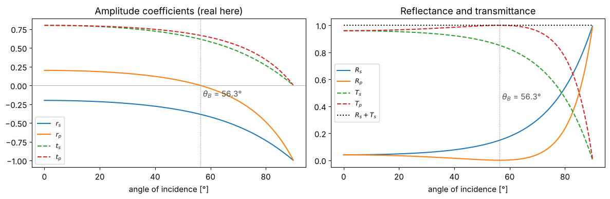
Different Fresnel formulas hold for s polarization (E perpendicular to the plane of incidence) and p polarization (E in the plane of incidence). At the Brewster angle \(\theta_B = \arctan(n_2/n_1)\), \(r_p\) vanishes: reflected and refracted beams are perpendicular to each other, and the dipoles in the glass do not radiate in the direction of the reflected beam. This is why light reflected at \(\theta_B\) is purely s polarized.

Energy conservation \(R + T = 1\) holds with \(T = \frac{\mathrm{Re}(n_2\cos\theta_2)}{\mathrm{Re}(n_1\cos\theta_1)}|t|^2\), not with \(|t|^2\) alone.

n1, n2 = 1.0, 1.5
theta = np.linspace(0, 89.9, 900)*deg
theta_B = itf.brewster_angle(n1, n2)

fig, axes = plt.subplots(1, 2, figsize=(12, 4))
axes[0].plot(theta/deg, itf.r_s(theta, n1, n2).real, label="$r_s$")
axes[0].plot(theta/deg, itf.r_p(theta, n1, n2).real, label="$r_p$")
axes[0].plot(theta/deg, itf.t_s(theta, n1, n2).real, "--", label="$t_s$")
axes[0].plot(theta/deg, itf.t_p(theta, n1, n2).real, "--", label="$t_p$")
axes[0].axhline(0, color="0.6", lw=0.5)
axes[0].set_title("Amplitude coefficients (real here)")
axes[1].plot(theta/deg, itf.R_s(theta, n1, n2), label="$R_s$")
axes[1].plot(theta/deg, itf.R_p(theta, n1, n2), label="$R_p$")
axes[1].plot(theta/deg, itf.T_s(theta, n1, n2), "--", label="$T_s$")
axes[1].plot(theta/deg, itf.T_p(theta, n1, n2), "--", label="$T_p$")
axes[1].plot(theta/deg, itf.R_s(theta, n1, n2) + itf.T_s(theta, n1, n2), "k:", label="$R_s + T_s$")
axes[1].set_title("Reflectance and transmittance")
for ax in axes:
    ax.axvline(theta_B/deg, color="0.5", lw=0.8, ls=":")
    ax.text(theta_B/deg + 1, -0.15 if ax is axes[0] else 0.45, f"$\\theta_B$ = {theta_B/deg:.1f}°", color="0.3")
    ax.set_xlabel("angle of incidence [°]"); ax.legend(fontsize=9)
fig.tight_layout()

2. Glass → air: total internal reflection and the evanescent wave

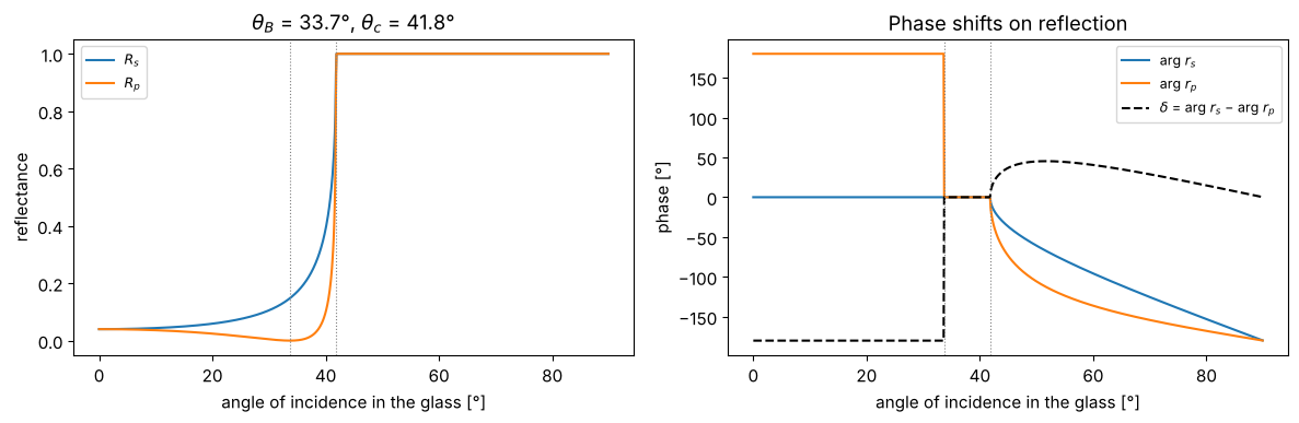
Above the critical angle \(\theta_c = \arcsin(n_2/n_1)\) everything is reflected, \(|r_s| = |r_p| = 1\). The reflection coefficients are then complex: the s and p components pick up different phase shifts. Linearly polarized light thus becomes elliptically polarized (Fresnel rhomb, see notebook 11).

n1, n2 = 1.5, 1.0
theta_c = np.real(itf.critical_angle(n1, n2))
theta_B = itf.brewster_angle(n1, n2)
rs, rp = itf.r_s(theta, n1, n2), itf.r_p(theta, n1, n2)

fig, axes = plt.subplots(1, 2, figsize=(12, 4))
axes[0].plot(theta/deg, np.abs(rs)**2, label="$R_s$")
axes[0].plot(theta/deg, np.abs(rp)**2, label="$R_p$")
axes[0].set_ylabel("reflectance")
axes[1].plot(theta/deg, np.angle(rs)/deg, label="arg $r_s$")
axes[1].plot(theta/deg, np.angle(rp)/deg, label="arg $r_p$")
axes[1].plot(theta/deg, (np.angle(rs) - np.angle(rp))/deg, "k--", label="$\\delta$ = arg $r_s$ − arg $r_p$")
axes[1].set_ylabel("phase [°]")
for ax in axes:
    ax.axvline(theta_c/deg, color="0.5", lw=0.8, ls=":")
    ax.axvline(theta_B/deg, color="0.5", lw=0.8, ls=":")
    ax.set_xlabel("angle of incidence in the glass [°]"); ax.legend(fontsize=9)
axes[0].set_title(f"$\\theta_B$ = {theta_B/deg:.1f}°, $\\theta_c$ = {theta_c/deg:.1f}°")
axes[1].set_title("Phase shifts on reflection")
fig.tight_layout()

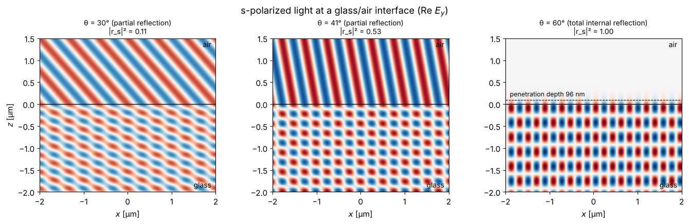
What does the field at the interface look like? For s polarization, \(E_y\) in the glass (\(z<0\)) is the sum of the incident and reflected waves, in the air (\(z>0\)) it is the transmitted wave

\[E_y = t_s\, e^{i(k_x x + k_{z,2} z)}, \qquad k_{z,2} = n_2 k_0 \cos\theta_2 .\]

Under total internal reflection, \(\cos\theta_2\) (from refracted_angle()) is purely imaginary with a positive imaginary part: the wave runs along the interface and decays exponentially in \(z\), with the penetration depth \(d = 1/\mathrm{Im}\,k_{z,2} = \lambda/(2\pi\sqrt{n_1^2\sin^2\theta - n_2^2})\). Shown is a snapshot \(\mathrm{Re}\,E_y\).

wl = 0.5
k0 = 2*np.pi/wl
xg = np.linspace(-2, 2, 400)
zg = np.linspace(-2, 1.5, 350)
Xg, Zg = np.meshgrid(xg, zg)

fig, axes = plt.subplots(1, 3, figsize=(14, 4.2))
for ax, th_deg in zip(axes, (30, 41, 60)):
    th = th_deg*deg
    th2 = itf.refracted_angle(th, n1, n2)
    kx = n1*k0*np.sin(th)
    kz1 = n1*k0*np.cos(th)
    kz2 = n2*k0*np.cos(th2)
    r, t = itf.r_s(th, n1, n2), itf.t_s(th, n1, n2)
    E = np.where(Zg < 0,
                 np.exp(1j*(kx*Xg + kz1*Zg)) + r*np.exp(1j*(kx*Xg - kz1*Zg)),
                 t*np.exp(1j*(kx*Xg + kz2*Zg)))
    ax.imshow(np.real(E), extent=(xg[0], xg[-1], zg[0], zg[-1]), cmap="RdBu_r", vmin=-2, vmax=2)
    ax.axhline(0, color="k", lw=1)
    label = "total internal reflection" if th > theta_c else "partial reflection"
    ax.set_title(f"θ = {th_deg}° ({label})\n|r_s|² = {abs(r)**2:.2f}", fontsize=10)
    ax.set_xlabel("$x$ [µm]")
    if th > theta_c:
        d = 1/np.imag(kz2)
        ax.axhline(d, color="k", ls="--", lw=0.8)
        ax.text(-1.9, d + 0.08, f"penetration depth {1000*d:.0f} nm", fontsize=9)
    ax.text(1.9, -1.9, "glass", ha="right", fontsize=10); ax.text(1.9, 1.3, "air", ha="right", fontsize=10)
axes[0].set_ylabel("$z$ [µm]")
fig.suptitle("s-polarized light at a glass/air interface (Re $E_y$)")
fig.tight_layout()

3. Reflection at metals

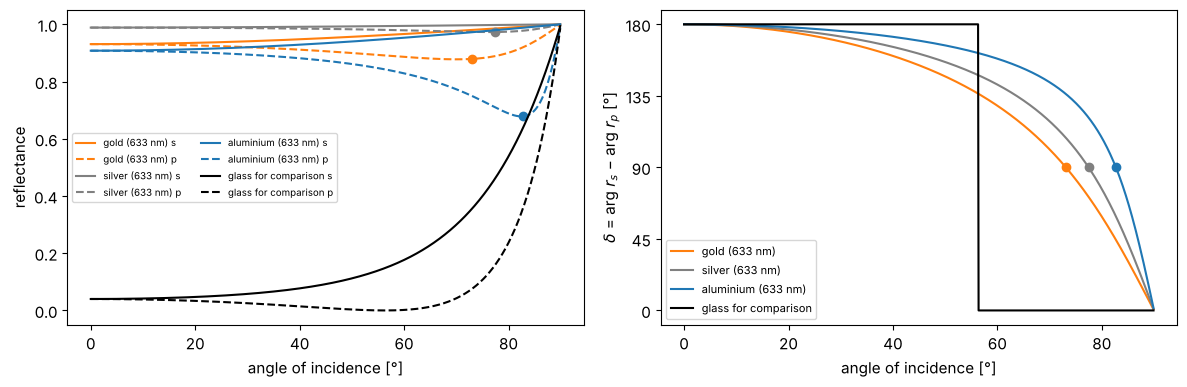
Metals have a large imaginary part of the refractive index. \(R_p\) then no longer has a true zero, but a minimum at the principal angle (pseudo-Brewster angle). Ellipsometry uses the phase difference \(\delta = \arg r_s - \arg r_p\) to determine \(n\) and \(\kappa\): it falls from \(180°\) (normal incidence, where \(r_p = -r_s\) in the Hecht convention) to \(0°\) (grazing incidence) and is exactly \(90°\) at the principal angle (dots). For glass, in contrast, it jumps from \(180°\) to \(0°\) at the Brewster angle.

metals = {"gold (633 nm)": 0.18 + 3.0j, "silver (633 nm)": 0.056 + 4.28j, "aluminium (633 nm)": 1.45 + 7.54j,
          "glass for comparison": 1.5 + 0j}
fig, axes = plt.subplots(1, 2, figsize=(12, 4))
for (name, nm), c in zip(metals.items(), ("C1", "0.5", "C0", "k")):
    axes[0].plot(theta/deg, itf.R_s(theta, 1.0, nm), color=c, ls="-", label=name + " s")
    axes[0].plot(theta/deg, itf.R_p(theta, 1.0, nm), color=c, ls="--", label=name + " p")
    delta = np.mod((np.angle(itf.r_s(theta, 1.0, nm)) - np.angle(itf.r_p(theta, 1.0, nm)))/deg + 1e-9, 360)
    axes[1].plot(theta/deg, delta, color=c, label=name)
    if nm.imag > 0:
        i90 = np.argmin(np.abs(delta - 90))
        axes[1].plot(theta[i90]/deg, 90, "o", color=c)
        axes[0].plot(theta[i90]/deg, itf.R_p(theta[i90], 1.0, nm), "o", color=c)
axes[0].set_ylabel("reflectance"); axes[0].legend(fontsize=7, ncol=2)
axes[1].set_ylabel("$\\delta$ = arg $r_s$ − arg $r_p$ [°]"); axes[1].legend(fontsize=8)
axes[1].set_yticks([0, 45, 90, 135, 180])
for ax in axes:
    ax.set_xlabel("angle of incidence [°]")
fig.tight_layout()

4. Thin films: the transfer matrix

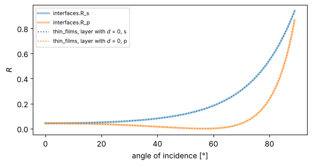
thin_films.r_t_coeffs() computes the amplitude coefficients of a layer stack (Zangwill/McLeod), R_T_A_coeffs() the intensities and the absorption \(A = 1 - R - T\). As a check: a layer of zero thickness must give the bare interface.

Note: thin_films refers \(r\) and \(t\) to the tangential field components. For p polarization, the sign of \(r_p\) therefore differs from the Hecht convention used in interfaces; the intensities are the same.

def stack_RTA(theta, wl, n, k, t, n_emb=1.0, n_sub=1.52, k_sub=0.0, pol="s", **kw):
    return tf.R_T_A_coeffs(theta, n, k, t, n_emb, 0.0, n_sub, k_sub, pol, wl, **kw)

th = np.linspace(0, 89, 90)*deg
R_stack = {pol: [stack_RTA(a, 0.55, [1.38], [0.0], [0.0], pol=pol)[0] for a in th] for pol in "sp"}
fig, ax = plt.subplots(figsize=(6.5, 3.5))
ax.plot(th/deg, itf.R_s(th, 1.0, 1.52), "C0", lw=3, alpha=0.4, label="interfaces.R_s")
ax.plot(th/deg, itf.R_p(th, 1.0, 1.52), "C1", lw=3, alpha=0.4, label="interfaces.R_p")
ax.plot(th/deg, R_stack["s"], "C0:", label="thin_films, layer with $d$ = 0, s")
ax.plot(th/deg, R_stack["p"], "C1:", label="thin_films, layer with $d$ = 0, p")
ax.set_xlabel("angle of incidence [°]"); ax.set_ylabel("$R$"); ax.legend(fontsize=8)
fig.tight_layout()

4.1 Colours of a soap film

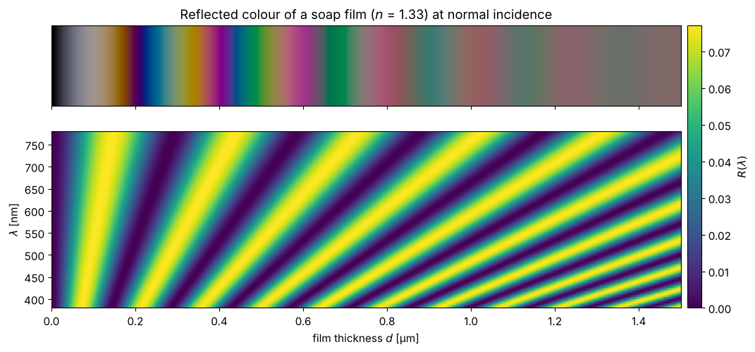
A water film (\(n = 1.33\)) in air preferentially reflects different wavelengths depending on its thickness. We compute \(R(\lambda)\) at normal incidence and convert the spectrum into sRGB colours with the CIE 1931 colour matching functions (analytic approximation by Wyman, Sloan and Shirley). Illumination: equal-energy white; the brightness is boosted for better visibility.

Very thin films appear black: the reflection at the front surface (low → high index) has a phase jump of \(\pi\) relative to the one at the back surface, so for \(d \to 0\) the two contributions cancel. With increasing thickness come white, yellow, purple, blue, … (Newton’s colour sequence), until the colours fade at a few µm because the interference maxima of many orders overlap in the visible spectrum.

def _g(lam, mu, s1, s2):
    s = np.where(lam < mu, s1, s2)
    return np.exp(-0.5*(lam - mu)**2/s**2)

def cie_xyz(lam_nm):
    xb = 1.056*_g(lam_nm, 599.8, 37.9, 31.0) + 0.362*_g(lam_nm, 442.0, 16.0, 26.7) - 0.065*_g(lam_nm, 501.1, 20.4, 26.2)
    yb = 0.821*_g(lam_nm, 568.8, 46.9, 40.5) + 0.286*_g(lam_nm, 530.9, 16.3, 31.1)
    zb = 1.217*_g(lam_nm, 437.0, 11.8, 36.0) + 0.681*_g(lam_nm, 459.0, 26.0, 13.8)
    return np.array([xb, yb, zb])

M_XYZ_to_sRGB = np.array([[3.2406, -1.5372, -0.4986], [-0.9689, 1.8758, 0.0415], [0.0557, -0.2040, 1.0570]])

def spectrum_to_rgb(lam_nm, S, gain=1.0):
    cmf = cie_xyz(lam_nm)
    XYZ = cmf @ S/np.sum(cmf[1])     # S = 1 everywhere -> Y = 1 (white)
    rgb = np.clip(gain*(M_XYZ_to_sRGB @ XYZ), 0, 1)
    return np.where(rgb <= 0.0031308, 12.92*rgb, 1.055*rgb**(1/2.4) - 0.055)  # sRGB gamma

lam = np.linspace(380, 780, 81)
d_vals = np.linspace(0, 1.5, 451)  # thickness in µm
R_map = np.array([[stack_RTA(0.0, l/1000, [1.33], [0.0], [d], n_sub=1.0)[0] for l in lam] for d in d_vals])
colors = np.array([spectrum_to_rgb(lam, R, gain=4.0) for R in R_map])

fig, axes = plt.subplots(2, 1, figsize=(12, 5.2), gridspec_kw={"height_ratios": [1, 2.2]}, sharex=True)
axes[0].imshow(colors[np.newaxis, :, :], extent=(d_vals[0], d_vals[-1], 0, 1), aspect="auto")
axes[0].set_yticks([]); axes[0].set_title("Reflected colour of a soap film ($n$ = 1.33) at normal incidence")
im = axes[1].imshow(R_map.T, extent=(d_vals[0], d_vals[-1], lam[0], lam[-1]), aspect="auto", cmap="viridis")
axes[1].set_xlabel("film thickness $d$ [µm]"); axes[1].set_ylabel("$\\lambda$ [nm]")
fig.colorbar(im, ax=axes, label="$R(\\lambda)$", fraction=0.03, pad=0.01)

<matplotlib.colorbar.Colorbar at 0x7f8ec5c9cd70>

4.2 Anti-reflection coating

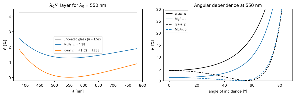
A layer of optical thickness \(\lambda_0/4\) makes the reflections at its front and back surfaces interfere with a phase difference of \(\pi\). They cancel completely when both are equally strong, i.e. for \(n_\text{layer} = \sqrt{n_\text{glass}}\). Real MgF\(_2\) (\(n = 1.38\)) comes close enough to reduce the reflection from 4.3 % to about 1.3 %.

lam = np.linspace(0.38, 0.78, 300)
lam0 = 0.55
fig, axes = plt.subplots(1, 2, figsize=(12, 4))
R_bare = [stack_RTA(0.0, l, [1.0], [0.0], [0.0])[0] for l in lam]
axes[0].plot(lam*1000, np.array(R_bare)*100, "k", label="uncoated glass ($n$ = 1.52)")
for n_c, lab in ((1.38, "MgF$_2$, $n$ = 1.38"), (np.sqrt(1.52), f"ideal, $n$ = $\\sqrt{{1.52}}$ = {np.sqrt(1.52):.3f}")):
    R = [stack_RTA(0.0, l, [n_c], [0.0], [lam0/(4*n_c)])[0] for l in lam]
    axes[0].plot(lam*1000, np.array(R)*100, label=lab)
axes[0].set_xlabel("$\\lambda$ [nm]"); axes[0].set_ylabel("$R$ [%]"); axes[0].legend(fontsize=9)
axes[0].set_title(f"$\\lambda_0/4$ layer for $\\lambda_0$ = {lam0*1000:.0f} nm")

th = np.linspace(0, 85, 86)*deg
for pol, ls in (("s", "-"), ("p", "--")):
    axes[1].plot(th/deg, [100*stack_RTA(a, lam0, [1.0], [0.0], [0.0], pol=pol)[0] for a in th], "k" + ls, label=f"glass, {pol}")
    axes[1].plot(th/deg, [100*stack_RTA(a, lam0, [1.38], [0.0], [lam0/(4*1.38)], pol=pol)[0] for a in th], "C0" + ls, label=f"MgF$_2$, {pol}")
axes[1].set_ylim(0, 30); axes[1].set_xlabel("angle of incidence [°]"); axes[1].set_ylabel("$R$ [%]")
axes[1].legend(fontsize=9); axes[1].set_title(f"Angular dependence at {lam0*1000:.0f} nm")
fig.tight_layout()

4.3 Bragg mirror

Alternating \(\lambda_0/4\) layers of high and low index material (TiO\(_2\)/SiO\(_2\)) reflect almost completely in a stop band around \(\lambda_0\). The reflectance grows with the number of pairs; the width of the stop band depends only on the index contrast. In frequency, it is symmetric about \(\omega_0\) with the relative width

\[\frac{\Delta\omega}{\omega_0} = \frac{4}{\pi}\arcsin\frac{n_H - n_L}{n_H + n_L},\]

so in wavelength it is asymmetric, with edges at \(\lambda_0/(1 \pm \Delta\omega/2\omega_0)\).

nH, nL = 2.35, 1.46
lam0 = 0.55
def bragg(N_pairs):
    n = [nH, nL]*N_pairs
    t = [lam0/(4*nH), lam0/(4*nL)]*N_pairs
    return n, [0.0]*len(n), t

lam = np.linspace(0.38, 0.85, 500)
fig, axes = plt.subplots(1, 2, figsize=(13, 4.2))
for N_pairs in (1, 2, 4, 8):
    n, k, t = bragg(N_pairs)
    axes[0].plot(lam*1000, [stack_RTA(0.0, l, n, k, t)[0] for l in lam], label=f"{N_pairs} pair" + ("s" if N_pairs > 1 else ""))
dw = 4/np.pi*np.arcsin((nH - nL)/(nH + nL))
axes[0].axvspan(lam0/(1 + dw/2)*1000, lam0/(1 - dw/2)*1000, color="0.9", zorder=-1, label="stop band (formula)")
axes[0].set_xlabel("$\\lambda$ [nm]"); axes[0].set_ylabel("$R$"); axes[0].legend(fontsize=9)
axes[0].set_title("TiO$_2$/SiO$_2$ Bragg mirror on glass, normal incidence")

n, k, t = bragg(8)
th = np.linspace(0, 80, 81)*deg
lam_map = np.linspace(0.38, 0.85, 240)
R_s = np.array([[stack_RTA(a, l, n, k, t, pol="s")[0] for l in lam_map] for a in th])
im = axes[1].imshow(R_s, extent=(lam_map[0]*1000, lam_map[-1]*1000, 0, 80), aspect="auto", cmap="magma")
axes[1].set_xlabel("$\\lambda$ [nm]"); axes[1].set_ylabel("angle of incidence [°]")
axes[1].set_title("8 pairs, s polarization: blue shift with angle")
fig.colorbar(im, ax=axes[1], label="$R$")
fig.tight_layout()

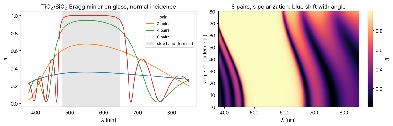
At oblique incidence the phase in each layer becomes \(k_0 n d\cos\theta\), the effective optical thickness decreases and the stop band moves to shorter wavelengths. This is behind the play of colours of many butterfly wings and beetle shells.

4.4 Thick plates: coherent or incoherent?

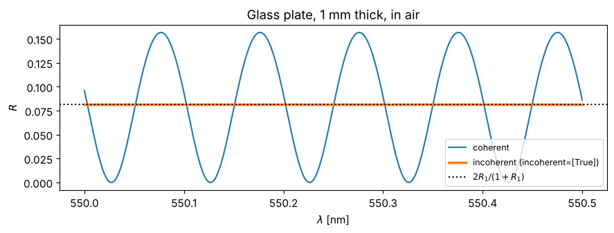
Strictly speaking, a 1 mm thick glass plate is a Fabry-Pérot resonator. But the interference fringes are so dense (\(\Delta\lambda = \lambda^2/(2nd) \approx 0.1\) nm) that every real spectrometer and every real light source averages them out. R_T_A_coeffs(..., incoherent=[True], N_phases=...) averages the intensities over the phase in the layer. The result is the sum of the reflections without interference, \(R = 2R_1/(1 + R_1)\).

lam = np.linspace(0.5500, 0.5505, 600)
d = 1000.0
R_coh = [stack_RTA(0.0, l, [1.52], [0.0], [d], n_sub=1.0)[0] for l in lam]
R_inc = [stack_RTA(0.0, l, [1.52], [0.0], [d], n_sub=1.0, incoherent=[True], N_phases=64)[0] for l in lam]
R1 = ((1.52 - 1)/(1.52 + 1))**2
fig, ax = plt.subplots(figsize=(9, 3.5))
ax.plot(lam*1000, R_coh, label="coherent")
ax.plot(lam*1000, R_inc, lw=2.5, label="incoherent (incoherent=[True])")
ax.axhline(2*R1/(1 + R1), color="k", ls=":", label="$2R_1/(1+R_1)$")
ax.set_xlabel("$\\lambda$ [nm]"); ax.set_ylabel("$R$"); ax.legend(fontsize=9)
ax.set_title("Glass plate, 1 mm thick, in air")
fig.tight_layout()

4.5 Thin metal films: reflection, transmission, absorption

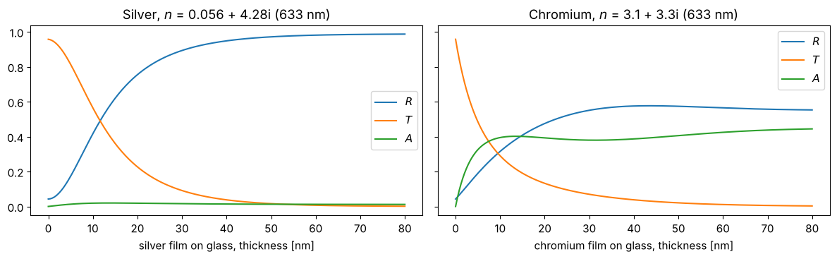
A silver film becomes a mirror after just a few tens of nm and absorbs hardly any light in the process (silver has a very small real part \(n\)). Chromium (\(n \approx 3.1 + 3.3i\)), on the other hand, absorbs strongly: from about 10 nm on, a chromium film swallows some 40 % of the light. Such films serve as neutral density filters.

d_vals = np.linspace(0, 0.08, 200)
fig, axes = plt.subplots(1, 2, figsize=(12, 3.8), sharey=True)
for ax, (name, n_m) in zip(axes, (("silver", 0.056 + 4.28j), ("chromium", 3.1 + 3.3j))):
    RTA = np.array([stack_RTA(0.0, 0.633, [n_m.real], [n_m.imag], [d]) for d in d_vals])
    for i, lab in enumerate(("$R$", "$T$", "$A$")):
        ax.plot(d_vals*1000, RTA[:, i], label=lab)
    ax.set_xlabel(f"{name} film on glass, thickness [nm]"); ax.legend()
    ax.set_title(f"{name.capitalize()}, $n$ = {n_m.real} + {n_m.imag}i (633 nm)")
fig.tight_layout()

References

• M. Born and E. Wolf, Principles of Optics, 7th ed., Cambridge University Press (1999).

• E. Hecht, Optics, 5th ed., Pearson (2017).

• A. Zangwill, Modern Electrodynamics, Cambridge University Press (2013).

• H. A. Macleod, Thin-Film Optical Filters, 3rd ed., Institute of Physics Publishing (2001).

• P. Yeh, Optical Waves in Layered Media, Wiley (1988).

• CIE 015:2018, “Colorimetry”, 4th ed., International Commission on Illumination (2018).