Resist model and swing curves

The lithography notebooks so far print with a constant threshold: the resist is removed wherever the dose times the image exceeds a threshold, optionally after a Gaussian blur. Real chemically amplified resists (the resists of KrF and ArF lithography) get there in steps, and each step leaves its mark on the printed feature:

step	model in pyoptics.litho.resist	parameters
image in the resist	intensity_in_resist(sim): \(\lvert E\rvert^2\) in an x–z cross section, with standing waves from the WaferStack	stack, focus
exposure	acid \(h_0 = 1 - e^{-C D I}\) (Dill C, no bleaching in DUV)	\(C\) [cm²/mJ], dose \(D\) [mJ/cm²]
post-exposure bake (PEB)	acid diffusion, neutralization by a base quencher, deprotection \(\partial_\tau m = -K h m\)	diffusion length \(\sigma\), quencher \(q_0\), amplification \(K\)
development	Mack rate \(r(m)\) and the development front from \(\lvert\nabla T\rvert = 1/r\) (fast marching)	\(r_\max\), \(r_\min\), \(n\), \(m_\mathrm{th}\), develop time
profile	CD at top, middle and bottom, sidewall angle, top loss

Before the chemistry, the optics of the film stack: the light reflected by the substrate interferes with the incoming light. That gives standing waves through the resist depth and, because the energy coupled into the resist depends on the thickness, swing curves. A bottom anti-reflective coating (BARC) suppresses both; wafer.swing_curve() and wafer.optimize_barc() compute them.

Contents:

1. Swing curves: reflectance and absorbed energy through resist thickness.

2. BARC optimization over the angles the illumination actually uses.

3. The image inside the resist, with and without BARC.

4. The resist chain step by step.

5. Standing waves in the profile and how the bake smooths them.

6. CD through dose: full model vs. threshold model, and the quencher.

7. Swing curves of the dose to clear and of the CD.

ArF immersion throughout: 193 nm, water (\(n = 1.437\)), NA 1.35, 45 nm lines and spaces with a y-polarized dipole on a 6 % attenuated PSM. All resist parameters are generic textbook values, not a calibrated resist.

import numpy as np
import matplotlib.pyplot as plt

from pyoptics.litho import (Illumination, LithoSimulation, MaskLayout, Projector, ThinMask,
                            WaferStack, resist, wafer)

plt.rcParams.update({"figure.dpi": 100, "font.size": 11})

wl, n_w, NA = 193.0, 1.437, 1.35
RESIST, BARC, SI = (1.70, 0.03), (1.82, 0.34), (0.883, 2.778)  # (n, k) at 193 nm, as in notebook 32
thickness = 100.0

sim = LithoSimulation(MaskLayout.lines_spaces(90.0, 45.0), ThinMask.att_psm(0.06),
                      Illumination.dipole(0.95, 0.7, polarization="y"), Projector(NA, wl, n=n_w))
bare = WaferStack(RESIST + (thickness,), substrate=SI, name="resist on Si")

1. Swing curves

A plane wave with transverse wave number \(k_0\,\mathrm{na}\) (na runs from 0 at normal incidence up to the NA) enters the stack. reflectance() is the reflectance of the whole stack, substrate_reflectance() the reflectance \(|r_b|^2\) of everything below the resist as seen from inside the resist, and absorbed() the fraction of the incident power absorbed in the resist,

\[ A = \frac{k_0\,\mathrm{Im}(n_r^2)}{n_\mathrm{medium}\cos\theta}\int_0^d |E(z)|^2\,dz, \]

integrated analytically (it equals \(1 - R - T\) when only the resist absorbs, which the tests check against pyoptics.thin_films). The swing period in thickness is \(\lambda/(2 n_r) \approx 57\) nm at normal incidence; oblique waves have a longer period.

Which angles matter? The image of the 90 nm pitch is made of the 0th and the first diffraction orders of each source point, at \(\mathrm{na} = |\mathrm{NA}\,\mathbf s + m\lambda/p\,\hat{\mathbf x}|\). With the dipole they all lie between na ≈ 0.9 and 1.3: hyper-NA lithography hits the wafer at steep angles only. The cell below collects these angles with the source weights (equal weights for the orders, a simplification) and averages over them.

ill, pitch = sim.illumination, 90.0
na_fill, w_fill = [], []
for m in (-1, 0, 1):
    na = np.hypot(NA*ill.s_x + m*wl/pitch, NA*ill.s_y)
    passed = na <= NA
    na_fill.append(na[passed]); w_fill.append(ill.weights[passed])
na_fill, w_fill = np.concatenate(na_fill), np.concatenate(w_fill)
print(f"{len(na_fill)} plane waves, na from {na_fill.min():.2f} to {na_fill.max():.2f}")

112 plane waves, na from 0.88 to 1.27

d = np.linspace(40, 220, 361)
fig, axes = plt.subplots(1, 2, figsize=(13, 4.2))
for na, w, ls, label in ((0.0, None, "-", "normal incidence"), (na_fill, w_fill, "--", "angles of the image")):
    sc = wafer.swing_curve(bare, d, wl, n_w, na=na, weights=w)
    axes[0].plot(d, sc.reflectance, ls, color="C0", label=label)
    axes[1].plot(d, sc.absorbed, ls, color="C0", label=label)
axes[0].set_ylabel("reflectance of the stack"); axes[1].set_ylabel("absorbed in the resist")
for ax in axes:
    ax.set_xlabel("resist thickness [nm]"); ax.legend(); ax.grid(alpha=0.3)
axes[0].set_title(f"resist on Si: period λ/(2n) = {wl/(2*RESIST[0]):.1f} nm")
axes[1].set_title("energy coupled into the resist")
plt.tight_layout()

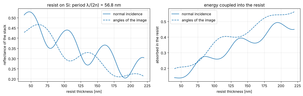
The absorbed energy, and with it the dose the resist needs, oscillates by more than a factor of 1.5 from one thickness to the next quarter period: on bare silicon a few nanometres of thickness variation over topography change the CD noticeably.

2. BARC optimization

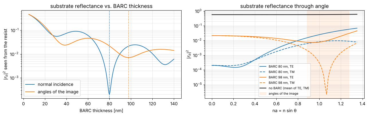
The BARC (here \(n = 1.82 + 0.34i\)) works by interference and absorption, so its best thickness depends on the angles. optimize_barc() scans the thickness and minimizes \(|r_b|^2\) averaged over the plane waves given. At NA 1.35 the optimum for normal incidence is not the optimum for the angles the image is made of, and no single layer reaches zero reflectance at those steep angles for both TE and TM.

tb = np.linspace(5, 140, 271)
best_0, R_0 = wafer.optimize_barc(bare, BARC, tb, wl, n_w, na=0.0)
best_fill, R_fill = wafer.optimize_barc(bare, BARC, tb, wl, n_w, na=na_fill, weights=w_fill)
print(f"normal incidence: {best_0:.1f} nm (|r_b|² = {R_0.min():.1e}), "
      f"angles of the image: {best_fill:.1f} nm (|r_b|² = {R_fill.min():.1e})")

fig, axes = plt.subplots(1, 2, figsize=(13, 4.2))
axes[0].plot(tb, R_0, label="normal incidence")
axes[0].plot(tb, R_fill, label="angles of the image")
for b, c in ((best_0, "C0"), (best_fill, "C1")):
    axes[0].axvline(b, color=c, ls=":")
axes[0].set_xlabel("BARC thickness [nm]"); axes[0].set_ylabel("$|r_b|^2$ seen from the resist")
axes[0].set_yscale("log"); axes[0].legend(); axes[0].set_title("substrate reflectance vs. BARC thickness")
na_fine = np.linspace(0, NA, 101)
for b, c in ((best_0, "C0"), (best_fill, "C1")):
    w = bare.with_(below=[BARC + (b,)])
    for pol, ls in (("TE", "-"), ("TM", "--")):
        axes[1].plot(na_fine, w.substrate_reflectance(na_fine, wl, n_w, pol), ls, color=c,
                     label=f"BARC {b:.0f} nm, {pol}")
axes[1].plot(na_fine, bare.substrate_reflectance(na_fine, wl, n_w), color="k", label="no BARC (mean of TE, TM)")
axes[1].axvspan(na_fill.min(), na_fill.max(), color="C1", alpha=0.1, label="angles of the image")
axes[1].set_yscale("log"); axes[1].set_xlabel("na = n sin θ"); axes[1].set_ylabel("$|r_b|^2$")
axes[1].legend(fontsize=8); axes[1].set_title("substrate reflectance through angle")
for ax in axes:
    ax.grid(alpha=0.3, which="both")
plt.tight_layout()

barc = bare.with_(below=[BARC + (best_fill,)], name=f"resist on {best_fill:.0f} nm BARC on Si")

normal incidence: 79.9 nm (|r_b|² = 2.0e-04), angles of the image: 97.7 nm (|r_b|² = 7.1e-03)

fig, ax = plt.subplots(figsize=(7, 4))
for w, c in ((bare, "C0"), (barc, "C2")):
    sc = wafer.swing_curve(w, d, wl, n_w, na=na_fill, weights=w_fill)
    ax.plot(d, sc.absorbed, color=c, label=w.name)
ax.set_xlabel("resist thickness [nm]"); ax.set_ylabel("absorbed in the resist (angle averaged)")
ax.legend(); ax.grid(alpha=0.3); ax.set_title("swing curve with and without BARC")
plt.tight_layout()

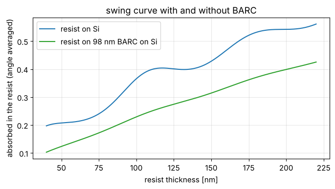
With the BARC the absorbed energy rises smoothly with thickness, the Beer law of the slightly absorbing resist; the swing is nearly gone.

3. The image inside the resist

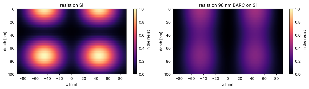
intensity_in_resist(sim) computes \(|E|^2\) across one period (x, periodic) and through the resist (z, cell centres), relative to the open frame intensity incident on the stack. On bare silicon the standing waves modulate the image through depth almost to zero; with the BARC a weak modulation from the residual reflectance at these steep angles is left, on top of the slow absorption decay.

lat_bare = resist.intensity_in_resist(sim.with_(wafer=bare), N_x=96, N_z=40)
lat_barc = resist.intensity_in_resist(sim.with_(wafer=barc), N_x=96, N_z=40)


def periodic(lat, values):
    # three periods of the grid, to show two periods centred on the feature
    x = np.concatenate([lat.x - lat.pitch, lat.x, lat.x + lat.pitch])
    return x, np.concatenate([values]*3, axis=1)


def show_xz(ax, lat, values, **kwargs):
    x, v = periodic(lat, values)
    im = ax.pcolormesh(x, lat.z, v, shading="nearest", **kwargs)
    ax.set_xlim(lat.center - lat.pitch, lat.center + lat.pitch)
    return im


fig, axes = plt.subplots(1, 2, figsize=(13, 3.8))
for ax, lat, w in zip(axes, (lat_bare, lat_barc), (bare, barc)):
    im = show_xz(ax, lat, lat.I, vmin=0, vmax=1.0, cmap="magma")
    ax.invert_yaxis(); ax.set_xlabel("x [nm]"); ax.set_ylabel("depth [nm]"); ax.set_title(w.name)
    fig.colorbar(im, ax=ax, label="I in the resist")
plt.tight_layout()

4. The resist chain step by step

A generic ArF resist: \(C = 0.05\) cm²/mJ, acid diffusion length 10 nm, amplification \(K = 2\), quencher 0.1 (relative to the acid generator), Mack development with \(r_\max = 100\) nm/s, \(r_\min = 0.1\) nm/s, \(n = 5\), \(m_\mathrm{th} = 0.5\) and 60 s develop time. dose_to_size() finds the dose that prints 45 nm at half the resist height.

model = resist.ResistModel(C=0.05, diffusion_length=10.0, amplification=2.0, quencher=0.1,
                           r_max=100.0, r_min=0.1, n=5.0, m_th=0.5, develop_time=60.0)
dose = model.dose_to_size(lat_barc, 45.0)
res = model.process(lat_barc, dose)
p = res.profile
print(f"dose to size: {dose:.1f} mJ/cm²")
print(f"CD top / middle / bottom: {p.cd_top:.1f} / {p.cd_middle:.1f} / {p.cd_bottom:.1f} nm, "
      f"sidewall angle {p.sidewall_angle:.1f}°, top loss {p.top_loss:.1f} nm")


def outline(ax, res, **kwargs):
    # the developed profile: contour of the arrival time at the develop time
    x, T = periodic(res.latent, res.arrival)
    kwargs.setdefault("colors", "w")
    ax.contour(x, lat.z, T, levels=[res.develop_time], **kwargs)


fig, axes = plt.subplots(2, 3, figsize=(16, 7))
panels = [(res.acid_0, "acid after exposure", "viridis", None),
          (res.acid, "acid after the bake (diffusion, quencher)", "viridis", None),
          (res.inhibitor, "inhibitor m after the bake", "cividis", None),
          (np.log10(res.rate), "log10 development rate [nm/s]", "plasma", None),
          (res.arrival, "arrival time of the front [s]", "turbo", (0, 3*model.develop_time)),
          (res.resist.astype(float), "resist after development", "Greys", (0, 1.4))]
for ax, (v, title, cmap, lim) in zip(axes.flat, panels):
    im = show_xz(ax, res.latent, v, cmap=cmap, vmin=None if lim is None else lim[0],
                 vmax=None if lim is None else lim[1])
    ax.invert_yaxis(); ax.set_title(title, fontsize=10)
    fig.colorbar(im, ax=ax)
outline(axes[1, 1], res)
outline(axes[1, 2], res, colors="C3")
for ax in axes[1]:
    ax.set_xlabel("x [nm]")
for ax in axes[:, 0]:
    ax.set_ylabel("depth [nm]")
plt.tight_layout()

dose to size: 19.6 mJ/cm²
CD top / middle / bottom: 32.4 / 45.0 / 46.2 nm, sidewall angle 88.5°, top loss 6.0 nm

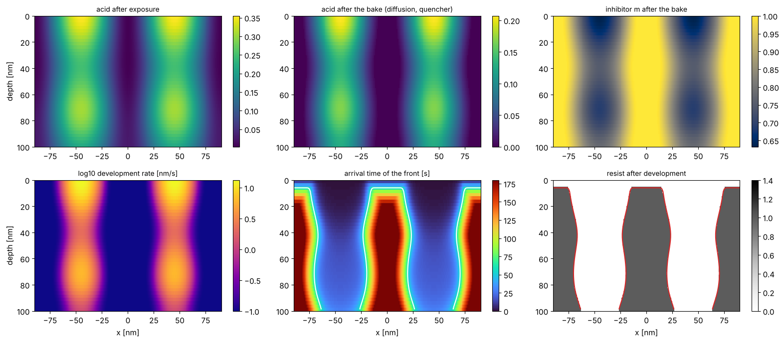
The quencher removes the acid tail in the dark regions (the bake panel is zero in the lines), the amplification turns a modest acid contrast into an inhibitor contrast, and the Mack rate turns that into more than two orders of magnitude in development rate. The arrival time shows how the front comes down through the spaces; where it arrives after 60 s, the resist stays. The lines lose \(r_\min \cdot 60\,\mathrm{s} = 6\) nm at the top (top loss), and their top corners are rounded: the developer works on them longest.

5. Standing waves in the profile

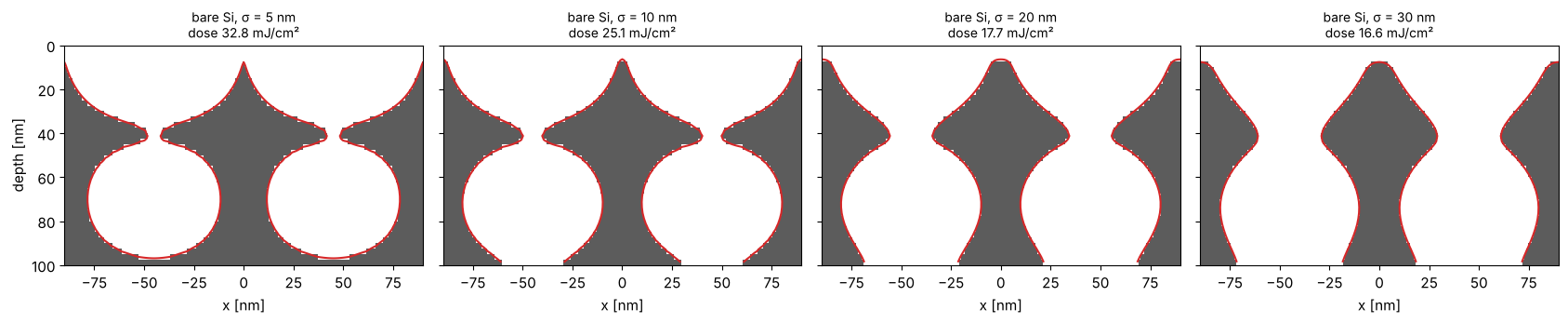
On bare silicon the standing waves are in the acid image as well. The bake diffuses the acid over \(\sigma\); the standing wave period is \(\lambda/(2n_r) = 57\) nm, so a diffusion length of 20 to 30 nm is needed to flatten them. With a short diffusion length the nodes of the standing wave develop slowly, and the profile has the typical ridges. Too much diffusion blurs the image across the 90 nm pitch as well. Each panel is at its own dose to size.

fig, axes = plt.subplots(1, 4, figsize=(17, 3.6), sharey=True)
for ax, sigma in zip(axes, (5.0, 10.0, 20.0, 30.0)):
    m = model.with_(diffusion_length=sigma)
    D = m.dose_to_size(lat_bare, 45.0)
    note = f"dose {D:.1f} mJ/cm²"
    r = m.process(lat_bare, D)
    show_xz(ax, r.latent, r.resist.astype(float), cmap="Greys", vmin=0, vmax=1.4)
    outline(ax, r, colors="C3")
    ax.set_title(f"bare Si, σ = {sigma:.0f} nm\n{note}", fontsize=10); ax.set_xlabel("x [nm]")
axes[0].set_ylabel("depth [nm]"); axes[0].invert_yaxis()
plt.tight_layout()

6. CD through dose

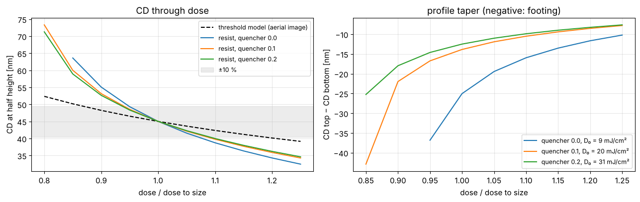
The full chain (with the BARC) against the constant threshold model of the aerial image, with the threshold chosen so that both print 45 nm at the nominal dose. Here the resist is more sensitive to dose than the threshold model: the acid diffusion lowers the image contrast, and the CD at half height sits at the waist of the profile. More quencher needs more dose but changes the CD slope little at this diffusion length; it does reduce the footing (right). Calibrated threshold models absorb such effects into a fitted blur and threshold, which is why they are fitted to resist data.

from pyoptics.litho import metrics

doses_rel = np.linspace(0.8, 1.25, 10)
u, I_aerial = sim.cut(N=801)
thr = 1.0/metrics.dose_to_size(u, I_aerial, 45.0, threshold=1.0)  # aerial threshold that prints 45 nm at relative dose 1
cd_thr = [metrics.threshold_cd(u, f*I_aerial, thr) for f in doses_rel]

fig, axes = plt.subplots(1, 2, figsize=(13, 4.2))
axes[0].plot(doses_rel, cd_thr, "k--", label="threshold model (aerial image)")
for q, c in ((0.0, "C0"), (0.1, "C1"), (0.2, "C2")):
    m = model.with_(quencher=q)
    D0 = m.dose_to_size(lat_barc, 45.0)
    profiles = [m.process(lat_barc, f*D0).profile for f in doses_rel]
    axes[0].plot(doses_rel, [pr.cd_middle for pr in profiles], color=c, label=f"resist, quencher {q}")
    axes[1].plot(doses_rel, [pr.cd_top - pr.cd_bottom for pr in profiles], color=c,
                 label=f"quencher {q}, D₀ = {D0:.0f} mJ/cm²")
axes[0].axhspan(45*0.9, 45*1.1, color="gray", alpha=0.15, label="±10 %")
axes[0].set_xlabel("dose / dose to size"); axes[0].set_ylabel("CD at half height [nm]")
axes[0].legend(fontsize=9); axes[0].set_title("CD through dose")
axes[1].set_xlabel("dose / dose to size"); axes[1].set_ylabel("CD top − CD bottom [nm]")
axes[1].legend(fontsize=9); axes[1].set_title("profile taper (negative: footing)")
for ax in axes:
    ax.grid(alpha=0.3)
plt.tight_layout()

7. Swing curves of the dose

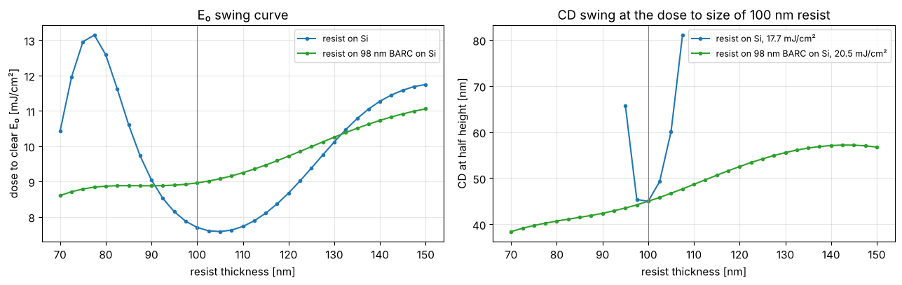
The classic swing curve is the dose to clear \(E_0\) of the open frame through resist thickness: open_frame_in_resist() gives the clear-field intensity through depth and ResistModel.dose_to_clear() the dose at which the development front reaches the bottom within the develop time. On bare silicon \(E_0\) swings, here with the longer period \(\lambda/(2 n_r\cos\theta_r) \approx 75\) nm of the steep dipole poles (\(\mathrm{na} \approx 1.1\), \(\theta_r \approx 40°\) in the resist) instead of 57 nm at normal incidence. With the BARC it only rises slowly (more resist to clear, more absorption). The CD swing at a fixed dose (right) follows: on bare silicon a few nanometres of thickness change the CD by several nanometres, or the space does not clear at half height at all (gaps in the curve).

m = model.with_(diffusion_length=20.0)
thick = np.linspace(70, 150, 33)
fig, axes = plt.subplots(1, 2, figsize=(13, 4.2))
for w, c in ((bare, "C0"), (barc, "C2")):
    E_0 = [m.dose_to_clear(resist.open_frame_in_resist(sim.with_(wafer=w.with_(thickness=t))))
           for t in thick]
    axes[0].plot(thick, E_0, "o-", ms=3, color=c, label=w.name)
    D = m.dose_to_size(resist.intensity_in_resist(sim.with_(wafer=w), N_x=96, N_z=40), 45.0)
    cds = [m.process(resist.intensity_in_resist(sim.with_(wafer=w.with_(thickness=t)), N_x=96, N_z=40), D)
           .profile.cd_middle for t in thick]
    axes[1].plot(thick, cds, "o-", ms=3, color=c, label=f"{w.name}, {D:.1f} mJ/cm²")
axes[0].set_ylabel("dose to clear E₀ [mJ/cm²]"); axes[0].set_title("E₀ swing curve")
axes[1].set_ylabel("CD at half height [nm]"); axes[1].set_title("CD swing at the dose to size of 100 nm resist")
for ax in axes:
    ax.axvline(thickness, color="gray", lw=0.8)
    ax.set_xlabel("resist thickness [nm]"); ax.legend(fontsize=9); ax.grid(alpha=0.3)
plt.tight_layout()

Summary

• wafer.swing_curve() gives reflectance, absorbed energy and substrate reflectance through resist thickness, averaged over the illumination angles; the swing period is \(\lambda/(2n_r)\).

• wafer.optimize_barc() picks the BARC thickness for the angles that matter: at NA 1.35 it differs from the normal incidence optimum.

• resist.intensity_in_resist() gives the image inside the resist, with the standing waves; resist.ResistModel runs exposure, PEB (diffusion, quencher, amplification) and Mack development with a fast marching development front, and reports CD at top, middle and bottom, sidewall angle and top loss.

• ResistModel.dose_to_clear() on open_frame_in_resist() gives the classic \(E_0\) swing curve; dose_to_size() the dose for a CD at any height of the profile.

• The bake smooths the standing waves once the diffusion length reaches about a third to a half of their period, at the price of image contrast across the pitch.

• Limitations: an x–z cross section (no diffusion along the lines), no bleaching, a generic uncalibrated resist, and fixed optical constants during exposure.

References

• T. A. Brunner, “Optimization of optical properties of resist processes”, Proc. SPIE 1466, 297 (1991).

• F. H. Dill, W. P. Hornberger, P. S. Hauge and J. M. Shaw, “Characterization of positive photoresist”, IEEE Trans. Electron Devices 22, 445-452 (1975).

• H. Ito and C. G. Willson, “Chemical amplification in the design of dry developing resist materials”, Polym. Eng. Sci. 23, 1012-1018 (1983).

• C. A. Mack, “Development of positive photoresists”, J. Electrochem. Soc. 134, 148-152 (1987).

• J. A. Sethian, “A fast marching level set method for monotonically advancing fronts”, Proc. Natl. Acad. Sci. USA 93, 1591-1595 (1996).

• C. Mack, Fundamental Principles of Optical Lithography: The Science of Microfabrication, Wiley (2007).