Beam shaping with the iterative Fourier transform algorithm (IFTA)

A diffractive optical element (DOE) is to shape a laser beam such that a given intensity pattern appears in the far field (or in the focal plane of a lens). The element may only change the phase. So we are looking for a phase \(\varphi(x, y)\) with

\[\big|\mathcal{F}\{A_\text{in}\, e^{i\varphi}\}\big|^2 \approx I_\text{target}.\]

The Gerchberg-Saxton algorithm jumps back and forth between object and image plane and imposes the known amplitude in each plane while keeping the phase. pyoptics.ifta implements this as the class GS, plus a variant with feedback (IFTA_HOO, hybrid output-output) and digitize_phase() for elements with few phase levels.

import numpy as np
import matplotlib.pyplot as plt
from scipy.ndimage import gaussian_filter

from pyoptics import ifta
from pyoptics.masks import mask_from_polygon
from pyoptics.utils import grid2d

plt.rcParams.update({"figure.dpi": 100, "image.origin": "lower", "font.size": 11})

1. Input beam and target pattern

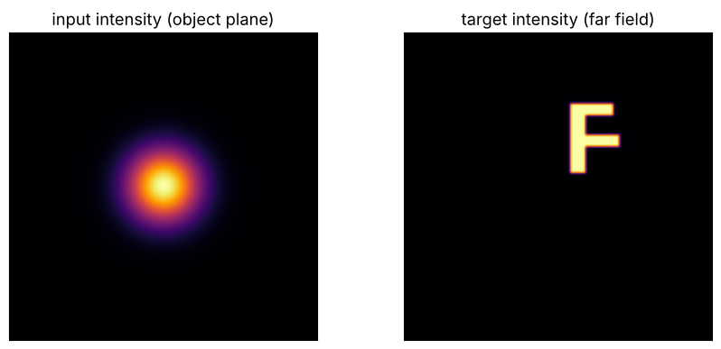
Input: a Gaussian beam. Target: the letter “F”, smoothed (sharp edges cannot be produced with a finite aperture), somewhat off-centre and normalized to the same energy as the input (Parseval). Coordinates in pixels.

N = 256
x, y, X, Y = grid2d(-N/2, N/2, -N/2, N/2, N)
A_in = np.exp(-(X**2 + Y**2)/(2*30**2))
I_in = A_in**2

F_poly_x = np.array([10, 22, 22, 50, 50, 22, 22, 45, 45, 10])
F_poly_y = np.array([10, 10, 32, 32, 42, 42, 58, 58, 68, 68])
target = mask_from_polygon(x, y, F_poly_x, F_poly_y).astype(float)
target = gaussian_filter(target, 1.0)
I_target = target*np.sum(I_in)/np.sum(target)  # same energy; FT_unitary conserves sum(|U|^2)
support = target > 0.5

fig, axes = plt.subplots(1, 2, figsize=(9, 4))
axes[0].imshow(I_in, cmap="inferno"); axes[0].set_title("input intensity (object plane)")
axes[1].imshow(I_target, cmap="inferno"); axes[1].set_title("target intensity (far field)")
for ax in axes:
    ax.set_xticks([]); ax.set_yticks([])
fig.tight_layout()

2. Gerchberg-Saxton

As figures of merit we use the efficiency (fraction of the energy inside the target region) and the non-uniformity (relative standard deviation of the intensity inside the letter). To record them in every iteration, we replace the algorithm’s stopping condition by a function that logs them, an example of the modular design of IFTABase.

def quality(img):
    I = np.abs(img)**2
    eta = I[support].sum()/I.sum()
    inner = target > 0.9
    nonunif = np.std(I[inner])/np.mean(I[inner])
    return eta, nonunif

def run_logged(alg_class, n_iter, start, **kwargs):
    alg = alg_class(I_in, I_target, n_iter, **kwargs)
    log = []
    def stop(curr_obj, curr_img, old_obj, old_img, i):
        # curr_img has already been overwritten with the target amplitude here, so
        # we compute the actual image from the current object:
        if i > 1:
            log.append(quality(alg.to_image_space(curr_obj, None, None, None, i)))
        return i > n_iter
    alg.stopping_condition = stop
    obj, img, _ = alg.iterate(start)
    return obj, alg.to_image_space(obj, None, None, None, 0), np.array(log)

rng = np.random.default_rng(3)
start = np.sqrt(I_target)*np.exp(2j*np.pi*rng.random((N, N)))
obj_gs, img_gs, log_gs = run_logged(ifta.GS, 100, start)

fig, axes = plt.subplots(1, 3, figsize=(14, 4.2))
im = axes[0].imshow(np.angle(obj_gs)*(A_in > 0.05*A_in.max()), cmap="twilight", vmin=-np.pi, vmax=np.pi)
axes[0].set_title("DOE phase (inside the beam)"); fig.colorbar(im, ax=axes[0], fraction=0.046)
axes[1].imshow(np.abs(img_gs)**2, cmap="inferno"); axes[1].set_title("resulting far field")
for ax in axes[:2]:
    ax.set_xticks([]); ax.set_yticks([])
axes[2].plot(log_gs[:, 0], label="efficiency")
axes[2].plot(log_gs[:, 1], label="non-uniformity")
axes[2].set_xlabel("iteration"); axes[2].set_ylim(0, 1.05); axes[2].legend()
axes[2].set_title("Convergence of Gerchberg-Saxton")
fig.tight_layout()

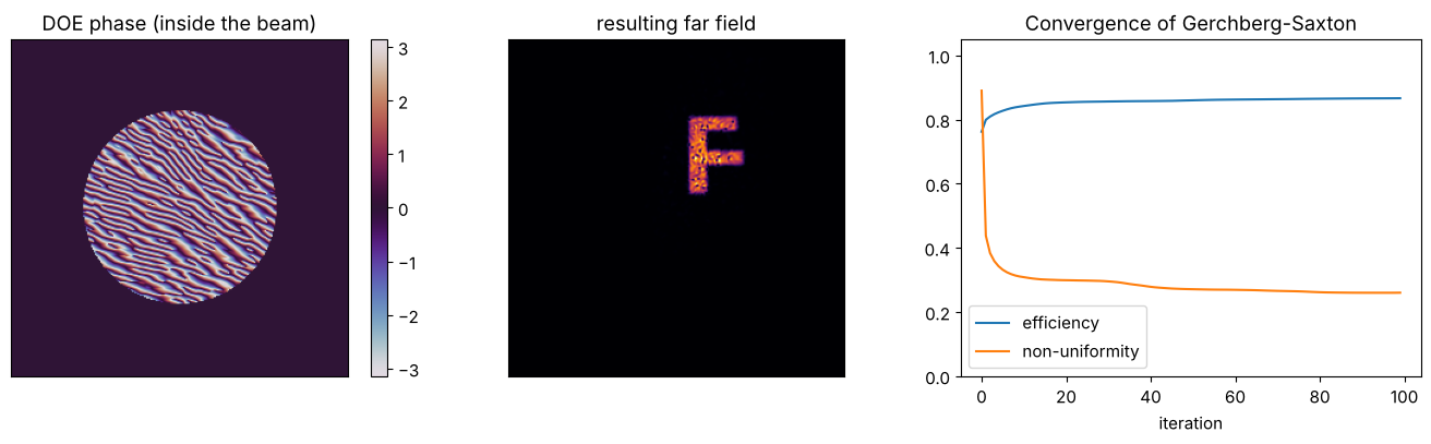
The far field is speckled: where the phase jumps inside the target region, zeros appear. Gerchberg-Saxton typically gets stuck in such a local minimum after a few iterations.

3. Escaping stagnation: feedback or a better start phase

IFTA_HOO mixes the image of the previous iteration with a correction term (parameter \(\beta = 0.9\)) to kick the algorithm out of local minima. Another, often more effective measure is a smooth start phase: a random start phase puts many phase vortices into the target region, whose zeros the algorithm cannot get rid of anymore. A quadratic start phase (like that of a lens), on the other hand, creates hardly any vortices.

quad_phase = 0.01*((X - 30)**2 + (Y - 39)**2)  # smooth, centred on the "F"
start_smooth = np.sqrt(I_target)*np.exp(1j*quad_phase)
obj_hoo, img_hoo, log_hoo = run_logged(ifta.IFTA_HOO, 100, start)
obj_sm, img_sm, log_sm = run_logged(ifta.GS, 100, start_smooth)

runs = (("GS, random start phase", img_gs, log_gs), ("HOO, random start phase", img_hoo, log_hoo),
        ("GS, smooth start phase", img_sm, log_sm))
fig, axes = plt.subplots(1, 4, figsize=(16, 4.2), gridspec_kw={"width_ratios": [1, 1, 1, 1.6]})
for ax, (name, img, log) in zip(axes, runs):
    I = np.abs(img)**2
    ax.imshow(I, cmap="inferno", vmax=np.percentile(I, 99.9))
    ax.set_xlim(N/2, N/2 + 64); ax.set_ylim(N/2, N/2 + 80); ax.set_xticks([]); ax.set_yticks([])
    ax.set_title(f"{name}\nη = {log[-1, 0]:.2f}, non-unif. = {log[-1, 1]:.2f}", fontsize=9)
    axes[3].plot(log[:, 1], label=name)
axes[3].set_yscale("log"); axes[3].set_xlabel("iteration"); axes[3].set_ylabel("non-uniformity")
axes[3].legend(fontsize=8); axes[3].set_title("Uniformity in the target region")
fig.tight_layout()

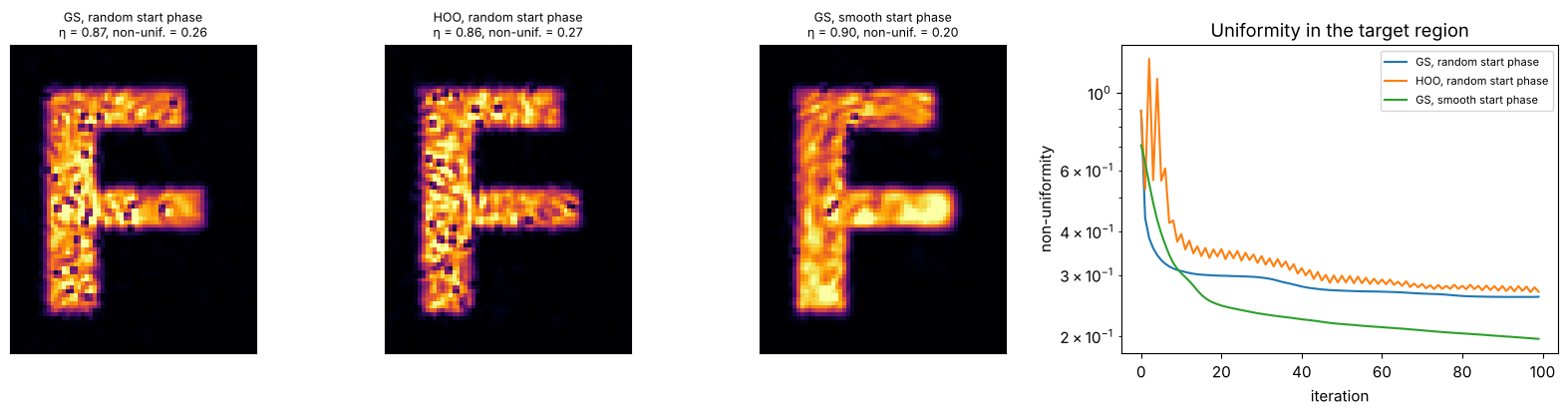
In this example, the feedback of HOO helps little, whereas the smooth start phase gives a visibly more uniform illumination at a somewhat higher efficiency. The speckle does not vanish completely: the target pattern is sharper than the finite size of the input beam allows.

4. Phase quantization: how many levels does the element need?

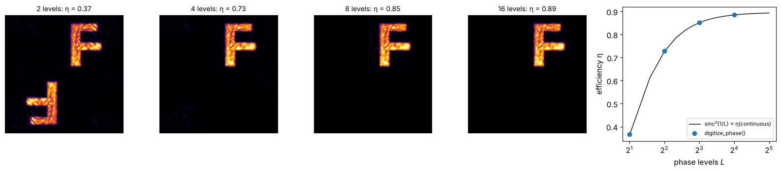
Lithographically fabricated DOEs have only \(2^n\) phase levels. digitize_phase() rounds the phase accordingly. With only two levels the transmission is real, so its far field is point symmetric: next to the “F”, its twin image rotated by \(180°\) appears, and the efficiency can be at most about 40 %. With 4, 8, 16 levels the result approaches the continuous element. Scalar theory gives \(\mathrm{sinc}^2(1/L)\) for the efficiency of the order the element “aims” at, with \(L\) levels.

levels = (2, 4, 8, 16)
fig, axes = plt.subplots(1, len(levels) + 1, figsize=(16, 3.6), gridspec_kw={"width_ratios": [1]*len(levels) + [1.3]})
etas = []
for ax, L in zip(axes, levels):
    obj_q = ifta.digitize_phase(obj_sm, L)
    img_q = ifta.FT_unitary(obj_q)
    eta, nonunif = quality(img_q)
    etas.append(eta)
    ax.imshow(np.abs(img_q)**2, cmap="inferno", vmax=np.percentile(np.abs(img_q)**2, 99.9))
    ax.set_title(f"{L} levels: η = {eta:.2f}", fontsize=10)
    ax.set_xlim(N/2 - 80, N/2 + 80); ax.set_ylim(N/2 - 80, N/2 + 80); ax.set_xticks([]); ax.set_yticks([])
Ls = np.arange(2, 33)
axes[-1].plot(Ls, np.sinc(1/Ls)**2*log_sm[-1, 0], "k-", lw=1, label="sinc²(1/L) × η(continuous)")
axes[-1].plot(levels, etas, "o", label="digitize_phase()")
axes[-1].set_xscale("log", base=2); axes[-1].set_xlabel("phase levels $L$"); axes[-1].set_ylabel("efficiency η")
axes[-1].legend(fontsize=8)
fig.tight_layout()

References

• R. W. Gerchberg and W. O. Saxton, “A practical algorithm for the determination of phase from image and diffraction plane pictures”, Optik 35, 237-246 (1972).

• J. R. Fienup, “Phase retrieval algorithms: a comparison”, Appl. Opt. 21, 2758-2769 (1982).

• F. Wyrowski and O. Bryngdahl, “Iterative Fourier-transform algorithm applied to computer holography”, J. Opt. Soc. Am. A 5, 1058-1065 (1988).

• F. Wyrowski, “Diffractive optical elements: iterative calculation of quantized, blazed phase structures”, J. Opt. Soc. Am. A 7, 961-969 (1990).

• O. Ripoll, V. Kettunen and H. P. Herzig, “Review of iterative Fourier-transform algorithms for beam shaping applications”, Opt. Eng. 43, 2549-2556 (2004).