Propagation with analytic phase: semi-analytical and homeomorphic Fourier transforms

A field behind a lens, near a point source or far from a waist has a strongly curved wavefront. Sampled as a complex array, its phase must change by less than \(\pi\) between neighbouring samples: a beam of width \(L\) with the radius of curvature \(R\) needs about \(L^2/(\lambda |R|)\) samples per axis, often thousands, although its amplitude is smooth and needs only a few dozen.

Wyrowski and coworkers (Wang et al. 2019, 2020) therefore write the field as

\[ u(x, y) = A(x, y)\, e^{i\psi(x, y)}, \]

with a smooth, sampled amplitude \(A\) and a phase \(\psi\) that is known analytically, and carry \(\psi\) through the operators of the propagation in closed form. pyoptics.analytic_phase does this for a separable quadratic phase \(\psi = \alpha_x x^2 + \alpha_y y^2 + \beta_x x + \beta_y y + \gamma\) (spherical or astigmatic wavefront, \(\alpha = k/(2R)\), with a tilt \(\beta\)):

Function	What it does
QuadraticPhaseField	amplitude, grid and analytic phase of a field or a spectrum
semi_analytical_FT(), inverse_semi_analytical_FT()	exact Fourier transforms that keep the quadratic phase analytic (SFT)
propagate()	angular spectrum (or Fresnel) propagation with SFTs: the same small \(N\) at any distance
tilted_plane()	the same onto a tilted plane
homeomorphic_FT()	pointwise (stationary phase) Fourier transform for any smooth phase (HFT)
geometric_propagation()	HFT, transfer function and inverse HFT: geometrical optics with amplitude transport

Semi-analytical Fourier transform. Completing the square gives, per axis and exactly,

\[ \int A(x)\, e^{i(\alpha x^2 + \beta x)}\, e^{-ikx}\,dx = e^{-i\kappa^2/(4\alpha)}\,(A * c)\!\left(\tfrac{\kappa}{2\alpha}\right), \qquad \kappa = k - \beta,\quad c(u) = e^{i\alpha u^2}. \]

The spectrum is again “amplitude times quadratic phase”: the phase \(-\kappa^2/(4\alpha)\) is analytic, the amplitude \(A * c\) lives on the grid \(k_j = \beta + 2\alpha x_j\) and is computed with FFTs, since the spectrum of the chirp \(c\) is known in closed form. The convolution with \(c\) is a mild blur where \(\alpha\) is large; for \(\alpha \to \infty\) it is the identity and the SFT becomes the pointwise (homeomorphic) transform.

Conventions as everywhere in pyoptics: fields vary as \(\exp(i(\mathbf k\cdot\mathbf r-\omega t))\), lengths are in µm.

import time
import warnings

import numpy as np
import matplotlib.pyplot as plt

from pyoptics.analytic_phase import (QuadraticPhaseField, semi_analytical_FT, propagate,
                                     tilted_plane, homeomorphic_FT, geometric_propagation)
from pyoptics.propagators import rayleigh_sommerfeld_I_TF
from pyoptics import tilted
from pyoptics.geometry import R_y
from pyoptics.utils import grid1d

plt.rcParams.update({"figure.dpi": 80, "font.size": 11, "figure.facecolor": "white",
                     "axes.facecolor": "#fcfcfb", "savefig.facecolor": "white",
                     "axes.grid": True, "grid.color": "0.88", "grid.linewidth": 0.6,
                     "axes.axisbelow": True, "axes.spines.top": False, "axes.spines.right": False,
                     "image.origin": "lower"})
CMAP = "magma_r"          # zero intensity is white
t_start = time.time()

WL = 0.5                   # wavelength [µm]
K = 2*np.pi/WL

# a lens with f = 8 mm and an aperture of 2 mm diameter (NA 0.125), soft (super-Gaussian) edge
f, a_ap, L = 8000.0, 1000.0, 2400.0

def aperture(x, y):
    R2 = x[None, :]**2 + y[:, None]**2
    return np.exp(-(R2/a_ap**2)**8)

def timed(func, *args, repeat=3, **kwargs):
    best = np.inf
    for _ in range(repeat):
        t = time.perf_counter()
        out = func(*args, **kwargs)
        best = min(best, time.perf_counter() - t)
    return out, best

1. The sampling problem

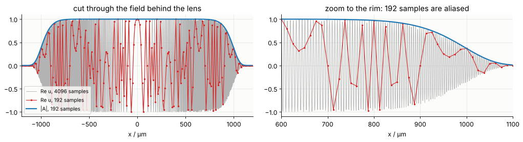
Behind the lens the phase \(-k r^2/(2f)\) changes fastest at the rim of the aperture, by \(k a\,\Delta x/f\) per sample. Sampling the complete field needs \(N \gtrsim L\,k\,(L/2)/(\pi f) = L^2/(\lambda f)\) samples over the window \(L\) for the phase alone, here 1440, plus those of the amplitude: about 1600 per axis (\(2.7\cdot 10^6\) samples). The amplitude alone is resolved by 192. Below: a cut through \(\mathrm{Re}\,u\) on 192 samples (aliased: the moiré has nothing to do with the field) and on 4096 samples, and the smooth amplitude that QuadraticPhaseField stores instead.

N = 192
x = grid1d(-L/2, L/2, N)
F0 = QuadraticPhaseField.from_curvature(aperture(x, x), x, x, WL, R=-f)
print("samples of the window:          ", N)
print("samples the full field needs:   ", F0.required_samples()[0])
print("chirp ratio rho = |a| N dx²/pi: {:.1f}  (> 1: the SFT is used)".format(F0.chirp_ratio()[0]))

x_fine = grid1d(-L/2, L/2, 4096)
fig, ax = plt.subplots(1, 2, figsize=(13, 3.6))
for a_ in ax:
    a_.plot(x_fine, np.cos(-K*x_fine**2/(2*f))*aperture(x_fine, np.zeros(1))[0], color="0.7",
            lw=0.8, label="Re u, 4096 samples")
    a_.plot(x, F0.field()[N//2].real, "C3.-", ms=4, lw=1, label="Re u, 192 samples")
    a_.plot(x, np.abs(F0.amplitude[N//2]), "C0", lw=2, label="|A|, 192 samples")
    a_.set(xlabel="x / µm")
ax[0].set(xlim=(-L/2, L/2), title="cut through the field behind the lens")
ax[1].set(xlim=(600, 1100), title="zoom to the rim: 192 samples are aliased")
ax[0].legend(loc="lower left", fontsize=9)
plt.tight_layout()

samples of the window:           192
samples the full field needs:    1632
chirp ratio rho = |a| N dx²/pi: 7.5  (> 1: the SFT is used)

2. The SFT is exact, and when it is needed

A Gaussian beam behind the lens has an analytic spectrum, \(\int e^{-a x^2} e^{-ikx}dx = \sqrt{\pi/a}\,e^{-k^2/(4a)}\) with \(a = 1/w^2 + i k/(2f)\). Its transform is computed on \(N\) samples over the same window, once with the SFT and once with the ordinary FFT of the complete field (mode="fft", here evaluated on the same output frequencies with a chirp-z transform).

The two branches are complementary. The chirp \(e^{i\alpha x^2}\) is sampled in \(x\) if \(\rho = |\alpha| N\Delta x^2/\pi < 1\), its counterpart \(e^{-i\nu^2/(4\alpha)}\) in the convolution of the SFT if \(\rho > 1\). With \(\Delta x = L/N\), \(\rho = |\alpha| L^2/(\pi N)\): the FFT needs many samples, the SFT works for few. mode="auto" picks the branch per axis.

w_g = 300.0
a_g = 1/w_g**2 + 1j*K/(2*f)
Ns = np.array([32, 48, 64, 96, 128, 192, 256, 384, 512, 768, 1024, 1536, 2048])
err = {"sft": [], "fft": []}
rho = []
for n_ in Ns:
    xg = grid1d(-L/2, L/2, n_)
    A_g = np.exp(-(xg[None, :]**2 + xg[:, None]**2)/w_g**2)
    Fg = QuadraticPhaseField.from_curvature(A_g, xg, xg, WL, R=-f)
    rho.append(Fg.chirp_ratio()[0])
    S = semi_analytical_FT(Fg, mode="sft")
    KX, KY = np.meshgrid(S.x, S.y)
    U_exact = np.pi/a_g*np.exp(-(KX**2 + KY**2)/(4*a_g))
    err["sft"].append(np.abs(S.field() - U_exact).max()/np.abs(U_exact).max())
    S_f = semi_analytical_FT(Fg, mode="fft", kx_out=S.x, ky_out=S.y)
    err["fft"].append(np.abs(S_f.field() - U_exact).max()/np.abs(U_exact).max())

N_rho1 = Ns[np.argmin(np.abs(np.array(rho) - 1))]
fig, ax = plt.subplots(figsize=(7.5, 4.2))
ax.loglog(Ns, err["sft"], "o-", label="SFT (analytic quadratic phase)")
ax.loglog(Ns, err["fft"], "s-", label="FFT of the complete field")
ax.axvline(K/(2*f)*L**2/np.pi, color="0.5", ls="--")
ax.text(K/(2*f)*L**2/np.pi*1.05, 1E-6, "ρ = 1", color="0.4")
ax.set(xlabel="samples N per axis", ylabel="max. relative error of the spectrum",
       title="Gaussian beam behind the lens (w = 300 µm, f = 8 mm)")
ax.legend()
plt.tight_layout()
for n_, e1, e2, r in zip(Ns, err["sft"], err["fft"], rho):
    print("N = {:5d}  rho = {:6.2f}   SFT {:.1e}   FFT {:.1e}".format(n_, r, e1, e2))

N =    32  rho =  45.00   SFT 1.2e-08   FFT 3.2e+00
N =    48  rho =  30.00   SFT 2.6e-08   FFT 7.9e+00
N =    64  rho =  22.50   SFT 4.1e-08   FFT 2.7e+00
N =    96  rho =  15.00   SFT 5.2e-08   FFT 2.8e+00
N =   128  rho =  11.25   SFT 4.1e-08   FFT 3.0e+00
N =   192  rho =   7.50   SFT 4.0e-08   FFT 1.5e+00
N =   256  rho =   5.62   SFT 4.2e-08   FFT 8.4e-01
N =   384  rho =   3.75   SFT 4.1e-08   FFT 3.3e-01
N =   512  rho =   2.81   SFT 4.0e-08   FFT 1.3e-01
N =   768  rho =   1.88   SFT 3.9e-08   FFT 1.0e-02
N =  1024  rho =   1.41   SFT 3.9e-08   FFT 3.1e-04
N =  1536  rho =   0.94   SFT 3.9e-08   FFT 4.2e-08
N =  2048  rho =   0.70   SFT 3.9e-08   FFT 4.0e-08

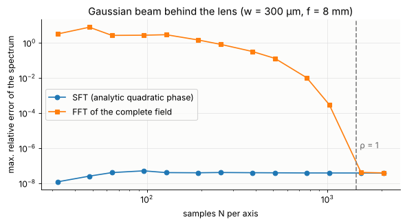
The SFT is exact from the smallest \(N\) on (the Gaussian amplitude is resolved by 32 samples) for all \(\rho\); the FFT needs \(\rho < 1\), i.e. \(N > 1440\). Near \(\rho = 1\) both work, which is where "auto" switches.

3. Through focus with 192 × 192 samples

propagate() does a forward SFT, multiplies the spectrum by \(e^{ik_z z}\) and transforms back. The paraxial part of the transfer function, \(e^{ikz}e^{-iz(k_x^2+k_y^2)/(2k)}\) (more precisely: the best fitting separable quadratic of \(k_z z\) over the spectrum), is added to the analytic quadratic phase of the spectrum; only the small non-paraxial remainder multiplies the sampled amplitude. The spectrum’s quadratic coefficient \(f/(2k) - z/(2k)\) vanishes at the focus, where the inverse transform turns into an ordinary FFT (or a chirp-z transform onto a chosen window). Away from the focus the output grid simply scales with the beam, \(x \to x\,(f - z)/f\).

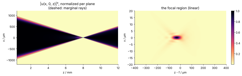
The side view below has 300 planes, each a full 2D propagation of the 192 × 192 field, evaluated on a fixed window (\(x\) = –1.2 … 1.2 mm, \(y = 0\)) and, on the right, on a 40 µm window around the focus.

zs = np.linspace(0.05*f, 1.5*f, 300)
x_side = np.linspace(-1200, 1200, 481)
x_near = np.linspace(-20, 20, 161)
zs_near = np.linspace(f - 400, f + 400, 161)
t = time.perf_counter()
side = np.array([propagate(F0, z, x_out=x_side, y_out=np.zeros(1)).intensity()[0] for z in zs])
near = np.array([propagate(F0, z, x_out=x_near, y_out=np.zeros(1)).intensity()[0] for z in zs_near])
t_side = time.perf_counter() - t
print("{} planes in {:.1f} s ({:.1f} ms per plane)".format(len(zs) + len(zs_near), t_side,
                                                         1E3*t_side/(len(zs) + len(zs_near))))

fig, ax = plt.subplots(1, 2, figsize=(13, 4.2))
ax[0].imshow(side.T/side.max(axis=1), extent=[zs[0]/1E3, zs[-1]/1E3, x_side[0], x_side[-1]],
             aspect="auto", cmap=CMAP, vmin=0, vmax=1)
ax[0].plot([0, f/1E3, 1.5*f/1E3], [a_ap, 0, -0.5*a_ap], "C0--", lw=0.8)
ax[0].plot([0, f/1E3, 1.5*f/1E3], [-a_ap, 0, 0.5*a_ap], "C0--", lw=0.8)
ax[0].set(xlabel="z / mm", ylabel="x / µm", xlim=(zs[0]/1E3, zs[-1]/1E3),
          title="|u(x, 0, z)|², normalized per plane\n(dashed: marginal rays)")
im = ax[1].imshow(near.T/near.max(), extent=[(zs_near[0] - f), (zs_near[-1] - f), x_near[0], x_near[-1]],
                  aspect="auto", cmap=CMAP)
ax[1].set(xlabel="z - f / µm", ylabel="x / µm", title="the focal region (linear)")
for a_ in ax:
    a_.grid(False)
plt.colorbar(im, ax=ax[1], fraction=0.046)
plt.tight_layout()

461 planes in 9.6 s (20.8 ms per plane)

Comparison with the angular spectrum method

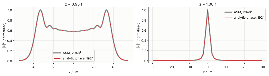
The reference is rayleigh_sommerfeld_I_TF() on the fully sampled field, 2048 × 2048 samples over the same window. Both are exact angular spectrum propagation; the table compares them at four planes, on the reference’s own grid points (the analytic-phase result is evaluated there with x_out, y_out).

Nr = 2048
xr = grid1d(-L/2, L/2, Nr)
U_ref0 = aperture(xr, xr)*np.exp(-1j*K*(xr[None, :]**2 + xr[:, None]**2)/(2*f))

rows = []
cuts = {}
for z in (0.5*f, 0.95*f, f, 1.3*f):
    (U_ref, _, _), t_ref = timed(rayleigh_sommerfeld_I_TF, U_ref0, xr, xr, z, WL, repeat=1)
    # window: the geometric beam (or 30 µm around the focus), every 4th reference sample
    half = max(30.0, 1.1*a_ap*abs(f - z)/f)
    sel = np.where(np.abs(xr) <= half)[0][::4 if half > 100 else 1]
    x_cmp = xr[sel]
    G, t_sft = timed(propagate, F0, z, x_out=x_cmp, y_out=x_cmp)
    ref = U_ref[np.ix_(sel, sel)]
    e = np.abs(G.field() - ref).max()/np.abs(ref).max()
    rows.append((z, t_ref, t_sft, e))
    cuts[z] = (x_cmp, np.abs(ref[len(sel)//2])**2, G.intensity()[len(sel)//2])

print(" z / mm   ASM 2048² [s]   analytic phase 192² [s]   max. rel. difference")
for z, t1, t2, e in rows:
    print("{:6.2f}   {:12.2f}    {:18.3f}       {:.1e}".format(z/1E3, t1, t2, e))

fig, ax = plt.subplots(1, 2, figsize=(13, 3.8))
for a_, z in zip(ax, (0.95*f, f)):
    xc, Ir, Ia = cuts[z]
    a_.plot(xc, Ir/Ir.max(), color="0.6", lw=4, label="ASM, 2048²")
    a_.plot(xc, Ia/Ir.max(), "C3", lw=1.2, label="analytic phase, 192²")
    a_.set(xlabel="x / µm", ylabel="|u|² (normalized)", title="z = {:.2f} f".format(z/f))
    a_.legend()
plt.tight_layout()

 z / mm   ASM 2048² [s]   analytic phase 192² [s]   max. rel. difference
  4.00           1.09                 0.029       5.6e-06
  7.60           0.93                 0.012       1.2e-06
  8.00           0.38                 0.017       3.8e-08
 10.40           0.45                 0.031       4.2e-06

The focus lies about 30 µm before \(z = f\): a quadratic phase is a paraxial lens, and exact (non-paraxial) propagation shows its spherical aberration, the marginal rays crossing the axis at \(f\cos\theta \approx f - 62\) µm. Both methods agree on this to about \(10^{-5}\) and better, with \(1/100\) of the samples and a fraction of the run time per plane. The remaining difference is the sampling of the amplitude’s soft edge and of the non-paraxial remainder of \(k_z z\): for higher NA this remainder grows (\(\propto z\,\mathrm{NA}^4\)), and propagate() issues a RuntimeWarning when it is no longer sampled (then more samples, or the spherical instead of the quadratic reference phase, are needed: the “generalized Debye integral” of Wang et al. 2020).

4. The pointwise limit: homeomorphic Fourier transform and geometrical optics

If the phase dominates, the Fourier integral is given by its stationary point alone: the sample at \(x\) is mapped to the spatial frequency \(k = \nabla\psi(x)\) and

\[ U(k) = A(x)\,\frac{2\pi}{\sqrt{|\det H|}}\,e^{i\pi\sigma(H)/4}\,e^{i(\psi(x) - k\cdot x)} \]

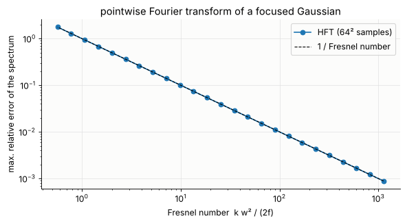
(\(H\): Hessian of \(\psi\), \(\sigma\): its signature). This homeomorphic Fourier transform (HFT) needs no FFT at all, only \(O(N)\) pointwise operations, and the phase may be any smooth function, given as an unwrapped array. Its error is of the order of the inverse Fresnel number: for the Gaussian behind the lens \(2f/(k w^2)\), the ratio of the beam’s own diffraction to the focusing.

fs = np.geomspace(500, 1E6, 25)
xg = grid1d(-L/2, L/2, 64)
XG, YG = np.meshgrid(xg, xg)
A_g = np.exp(-(XG**2 + YG**2)/w_g**2)
err_hft = []
for f_ in fs:
    kx, ky, U_amp, U_ph = homeomorphic_FT(A_g, -K*(XG**2 + YG**2)/(2*f_), xg, xg)
    a_ = 1/w_g**2 + 1j*K/(2*f_)
    U_ex = np.pi/a_*np.exp(-(kx**2 + ky**2)/(4*a_))
    err_hft.append(np.abs(U_amp*np.exp(1j*U_ph) - U_ex).max()/np.abs(U_ex).max())

fresnel = K*w_g**2/(2*fs)
fig, ax = plt.subplots(figsize=(7.5, 4.2))
ax.loglog(fresnel, err_hft, "o-", label="HFT (64² samples)")
ax.loglog(fresnel, 1/fresnel, "k--", lw=1, label="1 / Fresnel number")
ax.set(xlabel="Fresnel number  k w² / (2f)", ylabel="max. relative error of the spectrum",
       title="pointwise Fourier transform of a focused Gaussian")
ax.legend()
plt.tight_layout()

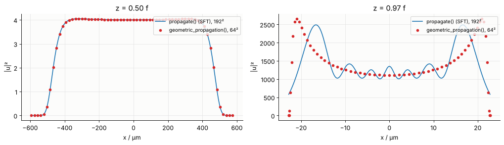
Chaining HFT, transfer function and inverse HFT gives geometric_propagation(): each sample travels along its ray to \(x + z\,\nabla\psi/k_z\), its amplitude scales with \(1/\sqrt{|\det(I - zHG)|}\) (the ray tube’s cross section; \(G\) is the Hessian of \(k_z\)), it collects the phase \(z k^2/k_z\) and \(-\pi/2\) per crossed focal line (Gouy phase). That is geometrical optics with amplitude transport, the limit in which Wyrowski’s field tracing connects to ray tracing. Below: the lens field at \(z = 0.5f\) and \(z = 0.97f\) by geometric propagation (64 × 64 samples, no FFT) and by propagate(). Far from focus they agree up to the diffraction at the soft edge; close to the focus the pointwise picture fails (the geometric intensity diverges at \(z = f\)).

xg = grid1d(-L/2, L/2, 64)
XG, YG = np.meshgrid(xg, xg)
A_ap = aperture(xg, xg)
psi_lens = -K*(XG**2 + YG**2)/(2*f)
fig, ax = plt.subplots(1, 2, figsize=(13, 3.8))
for a_, z in zip(ax, (0.5*f, 0.97*f)):
    xz, yz, ua, ph = geometric_propagation(A_ap, psi_lens, xg, xg, z, WL)
    x_line = np.linspace(xz[32].min(), xz[32].max(), 600)
    G = propagate(F0, z, x_out=x_line, y_out=np.zeros(1))
    a_.plot(x_line, G.intensity()[0], "C0", label="propagate() (SFT), 192²")
    a_.plot(xz[32], np.abs(ua[32])**2, "C3o", ms=4, label="geometric_propagation(), 64²")
    a_.set(xlabel="x / µm", ylabel="|u|²", title="z = {:.2f} f".format(z/f))
    a_.legend(loc="upper right", fontsize=9)
plt.tight_layout()

5. Tilted planes

Does this also work for tilted planes? Yes. Propagation onto a plane with a rotated normal is a coordinate transformation of the spectrum (Matsushima, Schimmel and Wyrowski 2003, notebook 03): the plane wave with wave vector \(\mathbf k\) reaches the plane with \(\hat{\mathbf k} = R^T\mathbf k\), and the spectrum must be resampled on a uniform \(\hat k\) grid, with the Jacobian \(k_z/\hat k_z\). In pyoptics.tilted this needs the complete field (fully sampled) and an interpolation of its spectrum, which for a curved beam is itself a strongly oscillating chirp (hence the padding there). With the analytic phase, analytic_phase.tilted_plane()

1. computes the spectrum with an SFT: smooth amplitude \(B(\mathbf k)\), analytic phase \(\tilde\psi(\mathbf k)\);

2. sets up a uniform grid of \(\hat{\mathbf k}\) over the rotated support, maps it back with \(\mathbf k = R\hat{\mathbf k}\) and interpolates only the smooth amplitude \(B\) there;

3. evaluates the phase \(\tilde\psi(\mathbf k) + \mathbf k\cdot\mathbf r_0\) exactly at the new points, keeps its best separable quadratic in \(\hat k\) (including the linear carrier, which Zhang et al. 2016 also treat analytically) as the analytic phase and samples only the small remainder;

4. transforms back with an inverse SFT in the plane’s own coordinates \((\hat x, \hat y)\).

The remainder that is not quadratic in \(\hat k\) (the tilt mixes \(k_x\) and \(k_z\), which gives coma-like cubic terms) must be sampled; N_out sets the samples of the target spectrum (default: twice the source) and a RuntimeWarning reports undersampling.

Example: a Gaussian beam (\(w\) = 40 µm) behind a lens with \(f\) = 200 µm (the full field needs about 480 samples per axis over the 220 µm window) and a plane through \(z_0\) = 120 µm, tilted by 45° about \(y\). Reference: tilted.tilted_plane(method="exact"), the exact non-uniform plane wave sum, on 512² samples.

w_t, f_t, z0, Lt = 40.0, 200.0, 120.0, 220.0
Rt = R_y(np.radians(45))
x_t_out = grid1d(-40, 40, 96)

xr_t = grid1d(-Lt/2, Lt/2, 512)
R2 = xr_t[None, :]**2 + xr_t[:, None]**2
U_t0 = np.exp(-R2/w_t**2)*np.exp(-1j*K*R2/(2*f_t))
t = time.perf_counter()
u_ref, _, _, _ = tilted.tilted_plane(U_t0, xr_t, xr_t, z0, WL, R=Rt, x_out=x_t_out, y_out=x_t_out,
                                     method="exact", remove_carrier=False)
t_ref = time.perf_counter() - t

x64 = grid1d(-Lt/2, Lt/2, 64)
A64 = np.exp(-(x64[None, :]**2 + x64[:, None]**2)/w_t**2)
F64 = QuadraticPhaseField.from_curvature(A64, x64, x64, WL, R=-f_t)
print("full field needs {} samples per axis, the analytic-phase field has 64".format(F64.required_samples()[0]))
T, t_ana = timed(tilted_plane, F64, z0, R=Rt, x_out=x_t_out, y_out=x_t_out, N_out=384)
e_ana = np.abs(T.field() - u_ref).max()/np.abs(u_ref).max()

# the standard method on the same 64² grid sees an aliased field
u_bad, _, _, _ = tilted.tilted_plane(F64.field(), x64, x64, z0, WL, R=Rt, x_out=x_t_out,
                                     y_out=x_t_out, method="exact", remove_carrier=False)
e_bad = np.abs(u_bad - u_ref).max()/np.abs(u_ref).max()
print("exact sum, 512²:            {:7.3f} s   (reference)".format(t_ref))
print("analytic phase, 64²:        {:7.3f} s   max. rel. difference {:.1e}".format(t_ana, e_ana))
print("exact sum on the 64² field:              max. rel. difference {:.1e}  (aliased input)".format(e_bad))

errs_nout = []
N_outs = [48, 64, 96, 128, 192, 256, 384, 512]
for n_ in N_outs:
    with warnings.catch_warnings():
        warnings.simplefilter("ignore")
        Tn = tilted_plane(F64, z0, R=Rt, x_out=x_t_out, y_out=x_t_out, N_out=n_)
    errs_nout.append(np.abs(Tn.field() - u_ref).max()/np.abs(u_ref).max())

fig, ax = plt.subplots(1, 3, figsize=(15, 4.2))
ext = [x_t_out[0], x_t_out[-1], x_t_out[0], x_t_out[-1]]
I_ref = np.abs(u_ref)**2
for a_, I, title in ((ax[0], I_ref, "exact sum, 512² source"),
                     (ax[1], T.intensity(), "analytic phase, 64² source")):
    im = a_.imshow(I/I_ref.max(), extent=ext, cmap=CMAP, vmin=0, vmax=1)
    a_.set(xlabel="x̂ / µm", ylabel="ŷ / µm", title=title + "\n|u|² on the plane tilted by 45°")
    plt.colorbar(im, ax=a_, fraction=0.046)
    a_.grid(False)
ax[2].semilogy(N_outs, errs_nout, "o-")
ax[2].set(xlabel="N_out (samples of the target spectrum)", ylabel="max. relative difference",
          title="convergence with the sampling\nof the non-quadratic remainder")
plt.tight_layout()

full field needs 549 samples per axis, the analytic-phase field has 64

exact sum, 512²:              2.163 s   (reference)
analytic phase, 64²:          0.077 s   max. rel. difference 2.6e-04
exact sum on the 64² field:              max. rel. difference 1.5e+00  (aliased input)

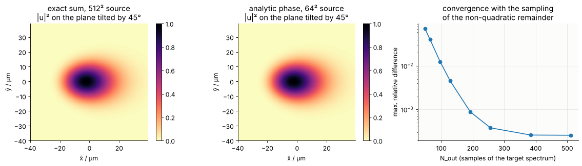
The footprint is stretched along \(\hat x\) (by \(1/\cos\theta\)) and asymmetric: the plane point \(\hat x\) lies at \(z = z_0 - \hat x\sin\theta\), so the half with \(\hat x < 0\) is closer to the focus and sees the smaller beam (a small effect here). With N_out=384 (the target spectrum, cheap) the analytic-phase result agrees with the exact sum to about \(10^{-4}\) from 64² instead of 512² source samples, about a hundred times faster, while the exact sum on the same 64² samples of the complete field is useless (aliased).

6. Notes

• What is analytic. A separable quadratic phase with a linear carrier. Rotated astigmatism (\(xy\) terms) and higher orders (e.g. spherical aberration, the non-paraxial part of a spherical wave) stay in the sampled amplitude, which must then resolve them. QuadraticPhaseField.from_field() splits a known curvature off a sampled field.

• Branches. Per axis, the SFT is used for \(\rho = |\alpha|N\Delta x^2/\pi \ge 1\) and the FFT (phase multiplied into the amplitude) otherwise. Behind an FFT step the amplitude carries the phase again; pass the desired output grid (x_out, y_out) to the transform instead of resampling afterwards (resample() warns in that case).

• Windows. The output grid of an SFT step is fixed by the input grid (\(k_j = \beta + 2\alpha x_j\)); arbitrary windows are obtained by interpolating the smooth amplitude. The source amplitude must decay inside its window: the chirp convolution spreads it slightly (zero padding pad=2 avoids wrap-around).

• Pointwise vs. semi-analytical. The HFT and geometric_propagation() are \(O(N)\) and accept any smooth phase, but are only valid at large Fresnel numbers away from foci and caustics. The SFT is exact everywhere, including the focus.

• Tilted planes. Implemented with the SFT (semi-analytically). The pointwise version would map each ray onto the tilted plane (ray tracing with amplitude transport) and is not implemented.

Tests: test/test_analytic_phase.py checks the SFT and the paraxial propagation of focused, astigmatic and tilted Gaussian beams against closed-form results (to \(10^{-8}\), before, at and behind the focus), the non-paraxial propagation against rayleigh_sommerfeld_I_TF(), the tilted plane against tilted.tilted_plane(), the HFT error against the inverse Fresnel number, and the ray mapping, Gouy phase and power conservation of geometric_propagation().

print("run time of the notebook: {:.0f} s".format(time.time() - t_start))

run time of the notebook: 27 s

References

• Z. Wang, S. Zhang, O. Baladron-Zorita, C. Hellmann and F. Wyrowski, “Application of the semi-analytical Fourier transform to electromagnetic modeling”, Opt. Express 27, 15335-15350 (2019).

• Z. Wang, O. Baladron-Zorita, C. Hellmann and F. Wyrowski, “Theory and algorithm of the homeomorphic Fourier transform for optical simulations”, Opt. Express 28, 10552-10571 (2020).

• Z. Wang, O. Baladron-Zorita, C. Hellmann and F. Wyrowski, “Generalized Debye integral”, Opt. Express 28, 24459-24470 (2020).

• F. Wyrowski and M. Kuhn, “Introduction to field tracing”, J. Mod. Opt. 58, 449-466 (2011).

• S. Zhang, D. Asoubar, C. Hellmann and F. Wyrowski, “Propagation of electromagnetic fields between non-parallel planes: a fully vectorial formulation and an efficient implementation”, Appl. Opt. 55, 529-538 (2016).

• K. Matsushima, H. Schimmel and F. Wyrowski, “Fast calculation method for optical diffraction on tilted planes by use of the angular spectrum of plane waves”, J. Opt. Soc. Am. A 20, 1755-1762 (2003).

• J. W. Goodman, Introduction to Fourier Optics, 4th ed., W. H. Freeman (2017).