Propagation onto tilted planes

Detectors, mirrors, wafers and fibre facets are often not perpendicular to the beam. The usual propagators connect parallel planes; pyoptics.tilted connects the plane \(z = 0\) with a plane through \(\mathbf r_0 = (0, 0, z_0)\) whose axes are the columns of a rotation matrix \(R\):

\[ \hat{\mathbf x} = R\,\mathbf e_x, \qquad \hat{\mathbf y} = R\,\mathbf e_y, \qquad \hat{\mathbf n} = R\,\mathbf e_z, \qquad \mathbf r(\hat x, \hat y) = \mathbf r_0 + \hat x\,\hat{\mathbf x} + \hat y\,\hat{\mathbf y}. \]

A plane wave \(e^{i\mathbf k\cdot\mathbf r}\) of the source spectrum arrives as \(e^{i\mathbf k\cdot\mathbf r_0}\,e^{i(\hat k_x \hat x + \hat k_y \hat y)}\) with the rotated wave vector \(\hat{\mathbf k} = R^T \mathbf k\). The field on the tilted plane is again a plane wave sum in the plane’s own coordinates, but over a non-uniform set of frequencies \(\hat k_x, \hat k_y\). Two methods evaluate it:

method	How	Cost
"exact"	the non-uniform sum itself; separable (one matrix product per spectrum row) for rotations about \(x\) or \(y\), finufft type 3 or a direct sum otherwise	\(O(N^3)\)
"rotation"	Matsushima (2003): uniform \(\hat k\) grid, map back with \(\mathbf k = R\hat{\mathbf k}\), interpolate the source spectrum, multiply by the Jacobian \(k_z/\hat k_z\), one inverse FFT	\(O(N^2\log N)\)

Function	What it does
tilted_plane()	scalar field on a tilted plane (or, with reverse=True, from a tilted plane to a parallel one)
vectorial_tilted_plane()	the same for \([E_x, E_y]\), components in the plane’s axes \(\hat E = R^T E\)
rotate_angular_spectrum()	the building block of "rotation"
tilted_beam_widths()	ISO 11146 widths on an inclined plane
power_flux()	power through a plane from the angular spectrum

Conventions as everywhere in pyoptics: fields vary as \(\exp(i(\mathbf k\cdot\mathbf r-\omega t))\), grids are centered (\(x = 0\) at index \(N/2\)), lengths are in units of the wavelength.

import time
import numpy as np
import matplotlib.pyplot as plt

from pyoptics.tilted import (tilted_plane, vectorial_tilted_plane, rotate_angular_spectrum,
                             tilted_beam_widths, power_flux, rotation_from_angles)
from pyoptics.geometry import R_y
from pyoptics.propagators import rayleigh_sommerfeld_I_TF, propagate_padded
from pyoptics.abcd import gaussian_field
from pyoptics.utils import grid1d, frequencies
from pyoptics.fft import FT, inv_FT

plt.rcParams.update({"figure.dpi": 100, "image.origin": "lower", "font.size": 11})
WL = 1.0
K = 2*np.pi/WL

def gaussian(x, y, w0, x0=0.0):
    return gaussian_field(x, y, 1j*np.pi*w0**2/WL, WL, x0=x0)

def gaussian_3d(P, w0):
    # paraxial Gaussian beam with its waist at z = 0 (with Gouy phase) at the points P
    z_R = np.pi*w0**2/WL
    return (gaussian_field(P[0], P[1], P[2] + 1j*z_R, WL)*np.exp(1j*K*P[2])
            *np.exp(-1j*np.arctan(P[2]/z_R)))

def plane_points(r0, R, x_t, y_t):
    X, Y = np.meshgrid(x_t, y_t)
    return np.asarray(r0, float)[:, None, None] + R[:, 0, None, None]*X + R[:, 1, None, None]*Y

1. Geometry: a Gaussian beam cut by inclined planes

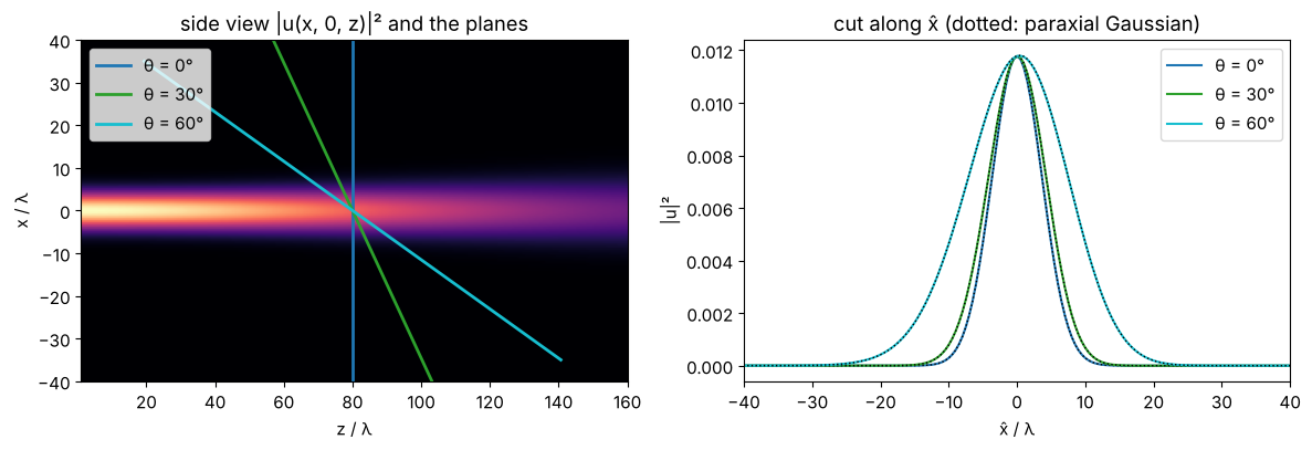
A Gaussian beam (\(w_0 = 6\lambda\), waist at \(z = 0\)) and three planes through \(z_0 = 80\lambda\), tilted about the \(y\) axis by \(\theta = 0°, 30°, 60°\). Left: the side view \(|u(x, 0, z)|^2\) from parallel angular spectrum propagation, with the planes. Right: \(|u|^2\) along the \(\hat x\) axis of each plane. The footprint stretches by \(1/\cos\theta\), and a tilted plane spans \(z_0 \mp \hat x\sin\theta\): its two halves see the beam at different distances, so the cut is slightly asymmetric.

N, L, w0, z0 = 256, 128.0, 6.0, 80.0
x = grid1d(-L/2, L/2, N); y = x.copy()
u0 = gaussian(x, y, w0)

z_side = np.linspace(1, 160, 160)
side = np.array([np.abs(propagate_padded(rayleigh_sommerfeld_I_TF, u0, x, y, z, WL)[0][N//2])**2
                 for z in z_side])

x_out = grid1d(-80, 80, 320)
fig, (ax1, ax2) = plt.subplots(1, 2, figsize=(12, 4.2))
ax1.imshow(side.T, extent=[z_side[0], z_side[-1], x[0], x[-1]], aspect="auto", cmap="magma")
for th, col in zip((0, 30, 60), ("C0", "C2", "C9")):
    R = R_y(np.radians(th))
    s = np.linspace(-70, 70, 2)
    ax1.plot(z0 + R[2, 0]*s, R[0, 0]*s, col, lw=2, label="θ = {}°".format(th))
    u_t, x_t, y_t, c = tilted_plane(u0, x, y, z0, WL, R=R, x_out=x_out, y_out=np.array([0.0]),
                                    method="exact")
    ax2.plot(x_t, np.abs(u_t[0])**2, col, label="θ = {}°".format(th))
    ax2.plot(x_t, np.abs(gaussian_3d(plane_points([0, 0, z0], R, x_t, [0.0]), w0)[0])**2,
             "k:", lw=1)
ax1.set(xlabel="z / λ", ylabel="x / λ", ylim=(-40, 40), title="side view |u(x, 0, z)|² and the planes")
ax1.legend(loc="upper left")
ax2.set(xlabel="x̂ / λ", ylabel="|u|²", xlim=(-40, 40), title="cut along x̂ (dotted: paraxial Gaussian)")
ax2.legend()
plt.tight_layout()

2. A beam on an inclined detector: intensity, phase and carrier

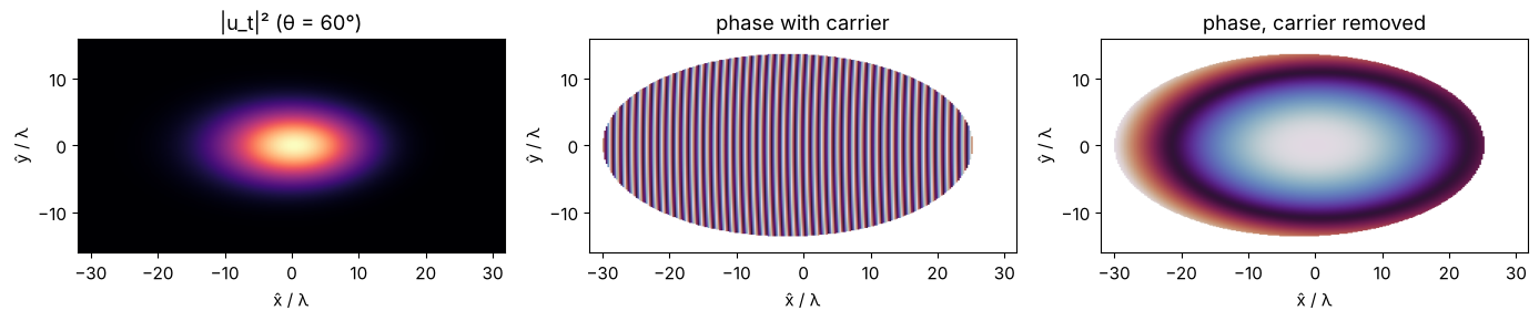
On a tilted plane the on-axis beam has the transverse wavenumber \(\hat k_x = -k\sin\theta\): the phase advances by \(2\pi\) every \(\lambda/\sin\theta\) along \(\hat x\), a fringe pattern that would need \(\Delta \hat x < \lambda/(2\sin\theta)\) to be sampled. With remove_carrier=True (default) this mean tilt is taken out and returned as k_carrier; the remaining phase is the curvature of the beam. The plots show \(|u_t|^2\) and the phase without and with the carrier, for \(\theta = 60°\) on a \(\lambda/4\) grid (where the carrier phase is still resolved).

R = R_y(np.radians(60))
xo = grid1d(-32, 32, 256)
u_c, x_t, y_t, _ = tilted_plane(u0, x, y, z0, WL, R=R, x_out=xo, y_out=xo/2, remove_carrier=False)
u_t, x_t, y_t, c = tilted_plane(u0, x, y, z0, WL, R=R, x_out=xo, y_out=xo/2)
print("carrier k_x^ = {:.4f}, -k sin(theta) = {:.4f}".format(c[0], -K*np.sin(np.radians(60))))

ext = [x_t[0], x_t[-1], y_t[0], y_t[-1]]
fig, axs = plt.subplots(1, 3, figsize=(14, 3.6))
axs[0].imshow(np.abs(u_t)**2, extent=ext, cmap="magma"); axs[0].set_title("|u_t|² (θ = 60°)")
mask = np.abs(u_t)**2 > 1E-3*np.max(np.abs(u_t)**2)
axs[1].imshow(np.where(mask, np.angle(u_c), np.nan), extent=ext, cmap="twilight")
axs[1].set_title("phase with carrier")
axs[2].imshow(np.where(mask, np.angle(u_t), np.nan), extent=ext, cmap="twilight")
axs[2].set_title("phase, carrier removed")
for ax in axs:
    ax.set(xlabel="x̂ / λ", ylabel="ŷ / λ")
plt.tight_layout()

carrier k_x^ = -5.4376, -k sin(theta) = -5.4414

Beam widths on inclined planes

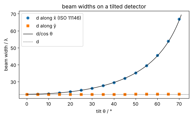
tilted_beam_widths() measures the ISO 11146 second moment widths of \(|u_t|^2\) in the plane’s coordinates. For a nearly collimated beam the width along \(\hat x\) grows as \(d/\cos\theta\) while \(d_{\hat y}\) stays: a tilted camera reports an elliptical beam. Dividing by \(1/\cos\theta\) recovers the true width (here \(w_0 = 8\lambda\) at \(z_0 = 200\lambda\), \(d = 2w(z_0)\)).

w0b, z0b = 8.0, 200.0
ub = gaussian(x, y, w0b)
d_true = 2*w0b*np.sqrt(1 + (z0b/(np.pi*w0b**2))**2)
thetas = np.arange(0, 71, 5)
dx, dy = [], []
for th in thetas:
    widths, *_ = tilted_beam_widths(ub, x, y, z0b, WL, R=R_y(np.radians(th)),
                                    x_out=grid1d(-180, 180, 512), y_out=grid1d(-50, 50, 128))
    phi = widths.phi % np.pi
    along_x = abs(np.cos(phi)) > abs(np.sin(phi))
    dx.append(widths.d_x if along_x else widths.d_y)
    dy.append(widths.d_y if along_x else widths.d_x)

fig, ax = plt.subplots(figsize=(6.5, 4))
ax.plot(thetas, dx, "o", label="d along x̂ (ISO 11146)")
ax.plot(thetas, dy, "s", label="d along ŷ")
tt = np.linspace(0, 71, 200)
ax.plot(tt, d_true/np.cos(np.radians(tt)), "k-", lw=1, label="d/cos θ")
ax.axhline(d_true, color="k", ls=":", lw=1, label="d")
ax.set(xlabel="tilt θ / °", ylabel="beam width / λ", title="beam widths on a tilted detector")
ax.legend()
plt.tight_layout()

3. Exact sum vs. spectrum rotation

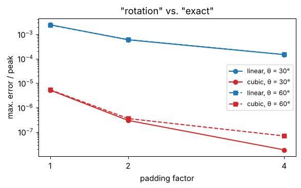
The "rotation" method interpolates the source spectrum. Its accuracy depends on the interpolation and on the zero padding of the source (which refines the spectrum). Here both methods for the beam of section 1 at \(\theta = 30°\) and \(60°\), relative to the peak. Linear interpolation converges with the square of the padding (\(2\cdot10^{-3} \to 1.7\cdot 10^{-4}\)), cubic interpolation is three orders of magnitude better at about twice the cost, and both are much faster than the exact sum.

xo = grid1d(-90, 90, 256)
rows = []
for th in (30, 60):
    R = R_y(np.radians(th))
    t = time.perf_counter()
    exact = tilted_plane(u0, x, y, z0 + 20, WL, R=R, x_out=xo, method="exact")[0]
    t_exact = time.perf_counter() - t
    for kind in ("linear", "cubic"):
        for p in (1, 2, 4):
            t = time.perf_counter()
            rot = tilted_plane(u0, x, y, z0 + 20, WL, R=R, x_out=xo, method="rotation",
                               kind=kind, pad=p)[0]
            dt = time.perf_counter() - t
            rows.append((th, kind, p, np.abs(rot - exact).max()/np.abs(exact).max(), dt, t_exact))

print("theta  kind    pad   error     t_rotation  t_exact")
for r in rows:
    print("{:4d}°  {:6s} {:3d}   {:.1e}   {:6.3f} s   {:5.2f} s".format(*r))

fig, ax = plt.subplots(figsize=(6, 3.8))
for th, m in ((30, "o-"), (60, "s--")):
    for kind, col in (("linear", "C0"), ("cubic", "C3")):
        e = [r[3] for r in rows if r[0] == th and r[1] == kind]
        ax.semilogy((1, 2, 4), e, m, color=col, label="{}, θ = {}°".format(kind, th))
ax.set(xlabel="padding factor", ylabel="max. error / peak", xticks=(1, 2, 4),
       title='"rotation" vs. "exact"')
ax.legend(fontsize=9)
plt.tight_layout()

theta  kind    pad   error     t_rotation  t_exact
  30°  linear   1   2.5e-03    0.018 s    0.72 s
  30°  linear   2   6.0e-04    0.028 s    0.72 s
  30°  linear   4   1.5e-04    0.082 s    0.72 s
  30°  cubic    1   5.2e-06    0.023 s    0.72 s
  30°  cubic    2   3.0e-07    0.059 s    0.72 s
  30°  cubic    4   1.9e-08    0.178 s    0.72 s
  60°  linear   1   2.4e-03    0.016 s    0.60 s
  60°  linear   2   6.1e-04    0.028 s    0.60 s
  60°  linear   4   1.5e-04    0.085 s    0.60 s
  60°  cubic    1   5.4e-06    0.024 s    0.60 s
  60°  cubic    2   3.6e-07    0.060 s    0.60 s
  60°  cubic    4   6.9e-08    0.223 s    0.60 s

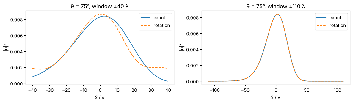
Pitfall: the window

The "rotation" result is periodic in the output window (it is an inverse FFT), the exact sum is not. If the beam does not fit into the window, it wraps around. At \(\theta = 75°\) the footprint is \(1/\cos 75° \approx 3.9\) times wider; on a window of \(\pm 40\lambda\) the far, wider half of the beam is cut off and its tail reappears on the other side (the exact sum simply shows the cut-out part). A window that holds the footprint cures it; the remaining difference of \(7\cdot 10^{-3}\) is the weak tail at the far edge (\(\hat x = -110\lambda\), \(z = 226\lambda\), where the beam is widest), which still wraps over to \(\hat x = +110\lambda\). Also, the plane must not cross the source plane inside the window (a ValueError says so).

R = R_y(np.radians(75))
fig, axs = plt.subplots(1, 2, figsize=(12, 3.6))
for ax, xo, title in ((axs[0], grid1d(-40, 40, 160), "window ±40 λ"), (axs[1], grid1d(-110, 110, 440), "window ±110 λ")):
    ex = tilted_plane(u0, x, y, 120.0, WL, R=R, x_out=xo, y_out=np.array([0.0]), method="exact")[0][0]
    # "rotation" needs an equidistant 2D window; take its centre row:
    ro = tilted_plane(u0, x, y, 120.0, WL, R=R, x_out=xo, y_out=grid1d(-32, 32, 128),
                      method="rotation")[0][64]
    ax.plot(xo, np.abs(ex)**2, label="exact")
    ax.plot(xo, np.abs(ro)**2, "--", label="rotation")
    ax.set(xlabel="x̂ / λ", ylabel="|u|²", title="θ = 75°, " + title)
    ax.legend()
    print("{}: max. difference {:.1e} of the peak".format(title, np.abs(ro - ex).max()/np.abs(ex).max()))
plt.tight_layout()

window ±40 λ: max. difference 3.0e-01 of the peak

window ±110 λ: max. difference 7.2e-03 of the peak

4. Why the Jacobian is mandatory

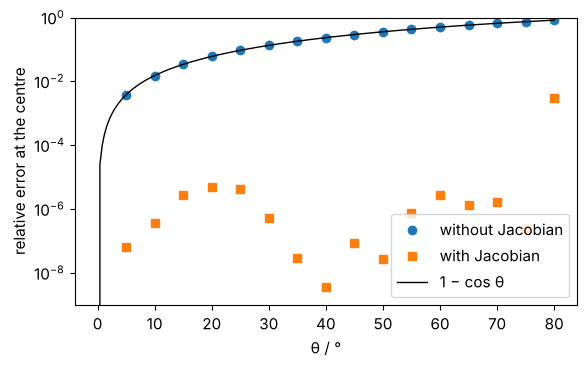
The rotated spectrum is a density: \(\hat A(\hat k_x, \hat k_y)\,d\hat k_x\,d\hat k_y = A(k_x, k_y)\,dk_x\,dk_y\). The area elements differ by the Jacobian \(|\partial(k_x, k_y)/\partial(\hat k_x, \hat k_y)| = k_z/\hat k_z\), which for an on-axis beam is \(1/\cos\theta\). Leaving it out (jacobian=False, only for this demonstration) scales the field by \(\cos\theta\): the error is \(1 - \cos\theta\), 50 % at 60°. Here the beam is rotated onto planes through its waist, where the field at the origin must stay the same.

F0 = FT(u0)
kx, ky = frequencies(x), frequencies(y)
thetas = np.arange(0, 81, 5)
err_with, err_without = [], []
for th in thetas:
    R = R_y(np.radians(th))
    grid = dict(kx_out=kx - K*np.sin(np.radians(th)), ky_out=ky)
    a = inv_FT(rotate_angular_spectrum(F0, kx, ky, K, R, **grid))[N//2, N//2]
    b = inv_FT(rotate_angular_spectrum(F0, kx, ky, K, R, jacobian=False, **grid))[N//2, N//2]
    err_with.append(abs(a/u0[N//2, N//2] - 1))
    err_without.append(abs(b/u0[N//2, N//2] - 1))

fig, ax = plt.subplots(figsize=(6, 3.8))
ax.plot(thetas, err_without, "o", label="without Jacobian")
ax.plot(thetas, np.array(err_with) + 1E-16, "s", label="with Jacobian")
tt = np.linspace(0, 80, 200)
ax.plot(tt, 1 - np.cos(np.radians(tt)), "k-", lw=1, label="1 − cos θ")
ax.set(yscale="log", ylim=(1E-9, 1), xlabel="θ / °", ylabel="relative error at the centre")
ax.legend()
plt.tight_layout()

5. What is conserved: flux, not \(\int |u|^2\)

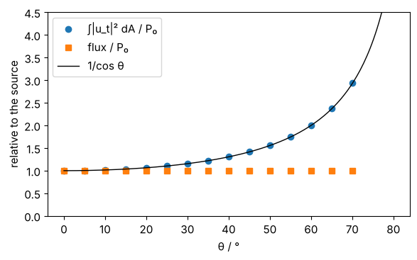
The integral of \(|u_t|^2\) over a tilted plane grows as \(1/\cos\theta\): the detector catches the same beam on a larger area. The power flux through the plane, \(P = \sum |A|^2 \hat k_z/k\) (power_flux()), is the same for every plane the beam crosses.

xo = grid1d(-180, 180, 512)
P0 = power_flux(ub, x, y, WL)
thetas = np.arange(0, 71, 5)
I_int, flux = [], []
for th in thetas:
    u_t, x_t, y_t, c = tilted_plane(ub, x, y, z0b, WL, R=R_y(np.radians(th)), x_out=xo,
                                    y_out=grid1d(-60, 60, 128), method="rotation")
    dA = (x_t[1] - x_t[0])*(y_t[1] - y_t[0])
    I_int.append(np.sum(np.abs(u_t)**2)*dA/P0)
    flux.append(power_flux(u_t, x_t, y_t, WL, k_carrier=c)/P0)

fig, ax = plt.subplots(figsize=(6, 3.8))
ax.plot(thetas, I_int, "o", label="∫|u_t|² dA / P₀")
ax.plot(thetas, flux, "s", label="flux / P₀")
ax.plot(tt, 1/np.cos(np.radians(tt)), "k-", lw=1, label="1/cos θ")
ax.set(xlabel="θ / °", ylabel="relative to the source", ylim=(0, 4.5))
ax.legend()
plt.tight_layout()
print("flux deviation max: {:.1e}".format(np.max(np.abs(np.array(flux) - 1))))

flux deviation max: 1.1e-06

6. The way back, and a tilted aperture

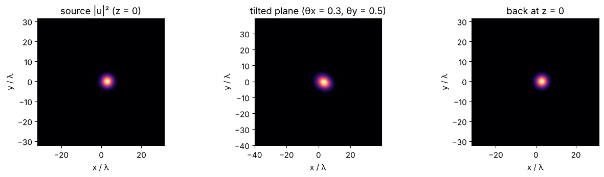
reverse=True makes the source the tilted plane: the field is given in the coordinates of a plane rotated by \(R\), and the target is the plane \(z = z_0\) of the unrotated frame. Internally this is the same propagation with \(R^{-1} = R^T\). Together with k_carrier_in (the carrier that was removed) it undoes a forward step: forward onto a plane tilted about \(x\) and \(y\), back to \(z = 0\).

xs = grid1d(-32, 32, 128)
us = gaussian(xs, xs, 4.0, x0=3.0)
R = rotation_from_angles(0.3, 0.5)
xt = grid1d(-40, 40, 160)
u_t, x_t, y_t, c = tilted_plane(us, xs, xs, 40.0, WL, R=R, x_out=xt, y_out=xt)
back, *_ = tilted_plane(u_t, x_t, y_t, -40.0, WL, R=R, reverse=True, k_carrier_in=c,
                        x_out=xs, y_out=xs, remove_carrier=False)
print("round trip error: {:.1e} of the peak".format(np.abs(back - us).max()/np.abs(us).max()))

fig, axs = plt.subplots(1, 3, figsize=(13, 3.6))
for ax, f, xx, yy, title in ((axs[0], us, xs, xs, "source |u|² (z = 0)"),
                             (axs[1], u_t, x_t, y_t, "tilted plane (θx = 0.3, θy = 0.5)"),
                             (axs[2], back, xs, xs, "back at z = 0")):
    ax.imshow(np.abs(f)**2, extent=[xx[0], xx[-1], yy[0], yy[-1]], cmap="magma")
    ax.set(title=title, xlabel="x / λ", ylabel="y / λ")
plt.tight_layout()

round trip error: 4.8e-13 of the peak

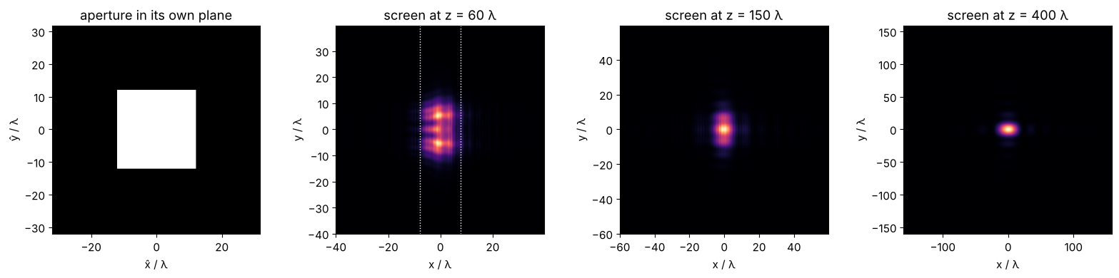
A square aperture (\(24\lambda \times 24\lambda\)) in a plane tilted by 50° about \(y\), lit by a plane wave travelling along \(z\). In the aperture’s coordinates the incident wave carries the carrier \(\hat k_x = -k\sin\theta\), which k_carrier_in passes on. The screens are parallel to \(z = 0\). Seen from the beam, the aperture is foreshortened by \(\cos 50° = 0.64\) in \(x\), and its left and right edges lie at different distances: the near field is asymmetric and the far field (here at \(z = 400\lambda\)) approaches that of a \(15.4\lambda \times 24\lambda\) rectangle. The screens must lie entirely in front of the (extended) aperture plane, here from \(z = 60\lambda\) on.

theta = np.radians(50)
R = R_y(theta)
xa = grid1d(-32, 32, 256)
Xa, Ya = np.meshgrid(xa, xa)
aperture = ((np.abs(Xa) <= 12) & (np.abs(Ya) <= 12)).astype(complex)
c_in = (-K*np.sin(theta), 0.0)

fig, axs = plt.subplots(1, 4, figsize=(16, 3.8))
axs[0].imshow(np.abs(aperture), extent=[xa[0], xa[-1], xa[0], xa[-1]], cmap="gray")
axs[0].set(title="aperture in its own plane", xlabel="x̂ / λ", ylabel="ŷ / λ")
for ax, d, half in ((axs[1], 60.0, 40), (axs[2], 150.0, 60), (axs[3], 400.0, 160)):
    xs_ = grid1d(-half, half, 256)
    u_s = tilted_plane(aperture, xa, xa, d, WL, R=R, reverse=True, k_carrier_in=c_in,
                       x_out=xs_, y_out=xs_, method="rotation", pad=2)[0]
    ax.imshow(np.abs(u_s)**2, extent=[xs_[0], xs_[-1], xs_[0], xs_[-1]], cmap="magma")
    ax.set(title="screen at z = {:g} λ".format(d), xlabel="x / λ", ylabel="y / λ")
axs[1].axvline(-12*np.cos(theta), color="w", ls=":", lw=1); axs[1].axvline(12*np.cos(theta), color="w", ls=":", lw=1)
plt.tight_layout()

7. Vector fields

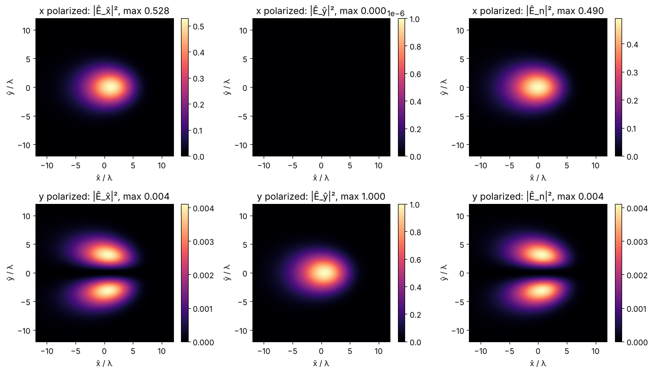
vectorial_tilted_plane() computes \(E_z\) of the source from \(\nabla\cdot\mathbf E = 0\), propagates all three Cartesian components and returns them in the plane’s axes: \(\hat E_{\hat x} = \mathbf E\cdot\hat{\mathbf x}\), \(\hat E_{\hat y} = \mathbf E\cdot\hat{\mathbf y}\) and the normal component \(\hat E_n = \mathbf E\cdot\hat{\mathbf n}\). For an \(x\) polarized beam on a plane tilted by \(\theta\) about \(y\) the field is mostly \(\hat E_{\hat x} = E_x\cos\theta\) and \(\hat E_n = E_x \sin\theta\); a \(y\) polarized beam stays tangential. A tight waist (\(w_0 = 1.5\lambda\)) also shows the small cross-polarized and longitudinal parts of the beam itself.

xv = grid1d(-24, 24, 192)
g = gaussian(xv, xv, 1.5)
theta = np.radians(45)
R = R_y(theta)
xo = grid1d(-16, 16, 160)
fig, axs = plt.subplots(2, 3, figsize=(13, 7.5))
for row, (pol, name) in enumerate(((np.array([1, 0]), "x"), (np.array([0, 1]), "y"))):
    field = np.stack([pol[0]*g, pol[1]*g], axis=-1)
    E_t, x_t, y_t, c = vectorial_tilted_plane(field, xv, xv, 20.0, WL, R=R, x_out=xo, y_out=xo)
    I_max = np.max(np.sum(np.abs(E_t)**2, axis=-1))
    for col, label in enumerate(("Ê_x̂", "Ê_ŷ", "Ê_n")):
        I = np.abs(E_t[..., col])**2/I_max
        im = axs[row, col].imshow(I, extent=[xo[0], xo[-1], xo[0], xo[-1]], cmap="magma",
                                  vmin=0, vmax=max(I.max(), 1E-6))
        axs[row, col].set(title="{} polarized: |{}|², max {:.3f}".format(name, label, I.max()),
                          xlabel="x̂ / λ", ylabel="ŷ / λ", xlim=(-12, 12), ylim=(-12, 12))
        plt.colorbar(im, ax=axs[row, col], fraction=0.046)
    if name == "x":
        centre = E_t[len(y_t)//2, len(x_t)//2]
        ratio = abs(centre[2]/centre[0])
plt.tight_layout()
print("x polarized, centre: |E_n/E_x^| = {:.4f}, tan(theta) = {:.4f}".format(ratio, np.tan(theta)))

x polarized, centre: |E_n/E_x^| = 1.0000, tan(theta) = 1.0000

8. Notes

• Method choice. By default "exact" is used for grids up to \(N = 256\) when the rotation is about \(x\) or \(y\) (or finufft is installed, or \(N \le 64\)), and "rotation" (cubic interpolation, 2× padding) otherwise. Both agree to about \(10^{-6}\) when the field fits into the window. Arbitrary, non-equidistant output points need "exact".

• Carrier. k_carrier is the power weighted mean of \((\hat k_x, \hat k_y)\); the true field is \(u_t\,e^{i(\hat k_{c,x}\hat x + \hat k_{c,y}\hat y)}\).

• Forward waves only. Plane waves that cross the target plane backwards (\(\hat k_z \le 0\), only for spectra with angles beyond \(90° - \theta\)) and evanescent waves are dropped.

• Windows and padding. The footprint stretches by \(1/\cos\theta\); choose x_out accordingly and pad the source when the beam spreads.

Tests: test/test_tilted.py checks \(\theta = 0\) against rayleigh_sommerfeld_I_TF(), plane waves and Gaussian beams against analytic fields at the plane’s 3D points, slice-by-slice propagation, the convergence of "rotation" to "exact", round trips, the way to parallel planes, flux conservation, the vectorial components and the beam widths.

References

• K. Matsushima, H. Schimmel and F. Wyrowski, “Fast calculation method for optical diffraction on tilted planes by use of the angular spectrum of plane waves”, J. Opt. Soc. Am. A 20, 1755-1762 (2003).

• J. W. Goodman, Introduction to Fourier Optics, 4th ed., W. H. Freeman (2017).

• ISO 11146-1:2021, “Lasers and laser-related equipment - Test methods for laser beam widths, divergence angles and beam propagation ratios - Part 1: Stigmatic and simple astigmatic beams”, International Organization for Standardization (2021).