Basis functions: Zernike, Legendre, Chebyshev and orthogonalized sets

Wavefronts, surface deviations and phase masks are usually described by a handful of coefficients in a basis set: \(W(x, y) = \sum_j c_j B_j(x, y)\). pyoptics.bases provides these sets with a common interface:

call	meaning
B(indices, coeffs)	evaluate \(\sum_j c_j B_j\) on the grid given at construction
B(indices, coeffs, x, y)	evaluate at scattered points
B.eval_single(j)	a single sampled basis function
B.mask	the support (circle, square, …)
B.normalization_factor(j)	the analytic norm \(\langle B_j \vert B_j \rangle\)
B.coeffs_from_field(W, indices, method)	expansion by least squares ("LSTSQ") or overlap integrals ("DI")
B.coeffs_from_scattered(x, y, data, indices)	least-squares fit to scattered samples

The concrete sets are FringeZernikes (circular apertures), LegendrePolynomials and ChebyshevPolynomials (rectangular apertures), plus the wrappers PresampledBasisSet, NumericallyOrthogonalized (Gram-Schmidt on an arbitrary aperture) and RescaledBasis.

This notebook is about the bases themselves: what they look like, in which sense they are orthogonal, and why orthogonality on the actual aperture matters. Notebook 15 uses the Zernikes for aberrations and the PSF.

import contextlib
import io
import time

import numpy as np
import matplotlib.pyplot as plt

from pyoptics.bases import (FringeZernikes, LegendrePolynomials, ChebyshevPolynomials,
                            PresampledBasisSet, NumericallyOrthogonalized, RescaledBasis,
                            fringe_to_n_m, fringe_zernike_R_nm, fringe_zernike_norm,
                            poly_basis_size)
from pyoptics.masks import circular_mask, annular_mask, mask_from_polygon
from pyoptics.utils import grid1d, scalar_product

plt.rcParams.update({"figure.dpi": 100, "image.origin": "lower", "font.size": 11})

def gram(funcs, x, y, weights=1.0):
    """Gram matrix G_ij = <B_i|B_j> = sum(w B_i B_j) dx dy of real sampled functions."""
    F = np.array([f.ravel() for f in funcs])
    dx, dy = x[1] - x[0], y[1] - y[0]
    return (F*np.ravel(weights*np.ones_like(funcs[0])))@F.T*dx*dy

def correlation(G):
    """|G_ij|/sqrt(G_ii G_jj): the cosine of the 'angle' between two functions.

    Exact zeros are raised to 1e-15 so that they show up on logarithmic colour scales."""
    d = np.sqrt(np.diag(G))
    return np.maximum(np.abs(G/np.outer(d, d)), 1e-15)

def show(ax, data, mask, extent, title, vmax=None, cmap="RdBu_r"):
    data = np.where(mask, data, np.nan)
    vmax = np.nanmax(np.abs(data)) if vmax is None else vmax
    im = ax.imshow(data, cmap=cmap, vmin=-vmax, vmax=vmax, extent=extent)
    ax.set_title(title, fontsize=9); ax.axis("off")
    return im

1. The Zernike pyramid

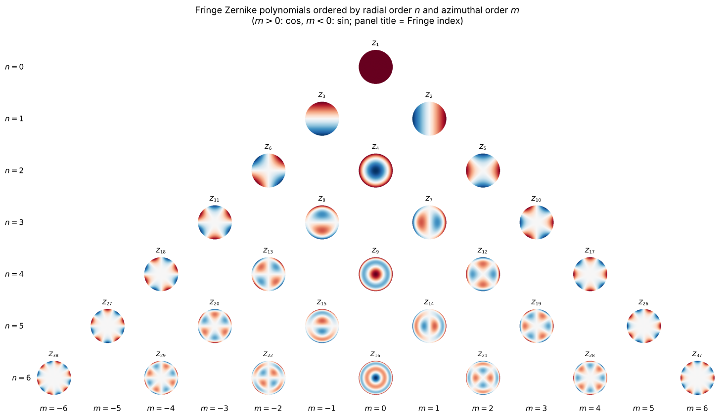
A Zernike polynomial is a radial polynomial times an azimuthal harmonic, \(Z_n^m(\rho, \varphi) = R_n^{|m|}(\rho)\,\{\cos, \sin\}(|m|\varphi)\), with \(n - |m|\) even. Arranged by radial order \(n\) (rows) and azimuthal order \(m\) (columns), they form a pyramid. The Fringe index \(j\) (shown in each panel) runs through the pyramid in a different order: it groups the functions by \((n + |m|)/2\), so that e.g. \(Z_9\) (primary spherical) comes before the trefoils \(Z_{10}, Z_{11}\), even though trefoil has \(n = 3\).

xg = grid1d(-1.02, 1.02, 161)
Zg = FringeZernikes(xg, xg)
mask_g = Zg.mask.astype(bool)
ext = (xg[0], xg[-1], xg[0], xg[-1])

lookup = {fringe_to_n_m(j): j for j in range(1, 50)}
n_max = 6
fig, axes = plt.subplots(n_max + 1, 2*n_max + 1, figsize=(15, 8.5))
for ax in axes.flat:
    ax.axis("off")
for n in range(n_max + 1):
    for m in range(-n, n + 1, 2):
        j = lookup.get((n, m))
        if j is None:
            continue
        ax = axes[n, m + n_max]
        show(ax, Zg.eval_single(j), mask_g, ext, f"$Z_{{{j}}}$", vmax=1)
for n in range(n_max + 1):
    axes[n, 0].text(-0.15, 0.5, f"$n = {n}$", transform=axes[n, 0].transAxes, ha="right", va="center")
for m in range(-n_max, n_max + 1):
    axes[-1, m + n_max].text(0.5, -0.25, f"$m = {m}$", transform=axes[-1, m + n_max].transAxes,
                             ha="center", va="top")
fig.suptitle("Fringe Zernike polynomials ordered by radial order $n$ and azimuthal order $m$\n"
             "($m > 0$: cos, $m < 0$: sin; panel title = Fringe index)", y=0.995)
fig.tight_layout()
fig.subplots_adjust(left=0.06)

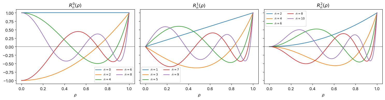
The radial parts \(R_n^m(\rho)\) all reach \(|R_n^m(1)| = 1\) at the rim; that is the Fringe normalization. Their number of zeros in \(0 < \rho < 1\) is \((n - m)/2\), and they oscillate faster near the rim than in the centre.

rho = np.linspace(0, 1, 400)
fig, axes = plt.subplots(1, 3, figsize=(15, 4), sharey=True)
for ax, m in zip(axes, (0, 1, 2)):
    for n in range(m, m + 9, 2):
        ax.plot(rho, fringe_zernike_R_nm(n, m, rho), label=f"$n={n}$")
    ax.set_title(f"$R_n^{{{m}}}(\\rho)$"); ax.set_xlabel("$\\rho$"); ax.axhline(0, color="k", lw=0.5)
    ax.legend(fontsize=8, ncol=2)
fig.tight_layout()

2. Orthogonality on the disk, and how well the grid reproduces it

On the unit disk,

\[\langle Z_i | Z_j \rangle = \int_\text{disk} Z_i Z_j \, dA = \delta_{ij}\, \frac{\pi (1 + \delta_{m0})}{2(n + 1)},\]

which normalization_factor() (or fringe_zernike_norm()) returns. On a grid, the integral becomes a sum and the circular edge a staircase, so orthogonality only holds approximately. The left panel shows the Gram matrix of \(Z_1 \dots Z_{36}\) on a 161 × 161 grid, normalized to unit diagonal; the off-diagonal elements are the discretization error. The right panel shows how that error and the error of the diagonal (compared with the analytic norm) shrink with the number of samples.

J36 = np.arange(1, 37)
G = gram([Zg.eval_single(j) for j in J36], xg, xg)

errs = []
Ns = (41, 81, 161, 321, 641)
for N in Ns:
    xs = grid1d(-1.02, 1.02, N)
    Zs = FringeZernikes(xs, xs)
    Gs = gram([Zs.eval_single(j) for j in J36], xs, xs)
    C = correlation(Gs)
    off = np.max(np.abs(C - np.diag(np.diag(C))))
    norm_err = np.max(np.abs(np.diag(Gs)/[fringe_zernike_norm(j) for j in J36] - 1))
    errs.append((off, norm_err))
errs = np.array(errs)

fig, axes = plt.subplots(1, 2, figsize=(12, 4.8))
im = axes[0].imshow((correlation(G)), cmap="magma", norm=plt.matplotlib.colors.LogNorm(1e-4, 1),
                    extent=(0.5, 36.5, 36.5, 0.5), origin="upper")
axes[0].set_title("$|\\langle Z_i|Z_j\\rangle| / \\sqrt{\\langle Z_i|Z_i\\rangle\\langle Z_j|Z_j\\rangle}$, 161 × 161 grid")
axes[0].set_xlabel("$j$"); axes[0].set_ylabel("$i$"); fig.colorbar(im, ax=axes[0])
axes[1].loglog(Ns, errs[:, 0], "o-", label="largest off-diagonal element")
axes[1].loglog(Ns, errs[:, 1], "s-", label="largest relative error of the norm")
axes[1].loglog(Ns, 3/np.array(Ns), "k--", lw=1, label="$\\propto 1/N$")
axes[1].set_xlabel("samples per axis $N$"); axes[1].legend(fontsize=9)
axes[1].set_title("Discretization error of the orthogonality, $j \\leq 36$")
fig.tight_layout()

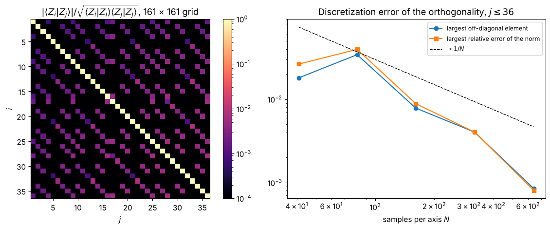
The error falls at least as fast as \(1/N\): it is dominated by the pixels along the staircase edge, whose share of the disk area scales like \(1/N\). Basis functions with high radial order are the worst, because they are largest at the rim.

3. Expanding a wavefront: least squares vs. overlap integrals

With an orthogonal basis, each coefficient can be computed independently as an overlap integral, \(c_j = \langle Z_j | W \rangle / \langle Z_j | Z_j \rangle\) (method="DI", using Simpson weights). Alternatively, all coefficients are fitted together by least squares (method="LSTSQ", the default), which minimizes the residual on the actual grid. We expand a smooth, non-polynomial “freeform” wavefront and watch the residual as the number of terms \(J\) grows.

XX, YY = np.meshgrid(xg, xg)
W = (np.exp(-((XX - 0.35)**2 + (YY + 0.2)**2)/(2*0.3**2)) + 0.4*np.sin(2.5*XX*YY + 0.5))*mask_g

def rms(a, mask):
    return np.sqrt(np.mean(a[mask]**2))

Js = np.array([4, 9, 16, 25, 36, 49, 64, 81, 100])
res = {"LSTSQ": [], "DI": []}
fits = {}
for J in Js:
    inds = np.arange(1, J + 1)
    for method in res:
        c = Zg.coeffs_from_field(W, inds, method=method)
        Wfit = Zg(inds, c)
        res[method].append(rms(W - Wfit, mask_g))
        if method == "LSTSQ":
            fits[J] = Wfit

fig = plt.figure(figsize=(15, 4.2))
gs = fig.add_gridspec(1, 5, width_ratios=[1, 1, 1, 1, 1.7])
vmax = np.max(np.abs(W))
show(fig.add_subplot(gs[0]), W, mask_g, ext, "wavefront $W$", vmax)
for k, J in enumerate((9, 36)):
    show(fig.add_subplot(gs[1 + k]), fits[J], mask_g, ext, f"fit, $J = {J}$", vmax)
show(fig.add_subplot(gs[3]), W - fits[36], mask_g, ext, "residual, $J = 36$ (×10)", vmax/10)
ax = fig.add_subplot(gs[4])
for method, r in res.items():
    ax.semilogy(Js, np.array(r)/rms(W, mask_g), "o-", label=method)
ax.set_xlabel("number of terms $J$"); ax.set_ylabel("rms residual / rms $W$"); ax.legend()
ax.set_title("Convergence of the Zernike expansion")
fig.tight_layout()

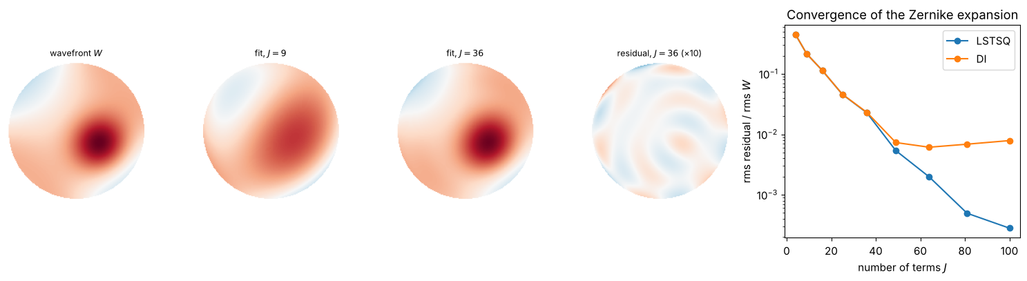
Both methods converge quickly for this smooth wavefront. Least squares is always at least as good, because it minimizes exactly the quantity that is plotted. The overlap integrals stall at the level of the discretization error from Section 2: on the grid, the Zernikes are not exactly orthogonal, and DI ignores that.

4. Rectangular apertures: Legendre and Chebyshev polynomials

For square or rectangular apertures (slit lamps, detectors, mask blanks), products of 1D polynomials \(P_n(x) P_m(y)\) are the natural choice. LegendrePolynomials and ChebyshevPolynomials use a single index \(j = 0, 1, 2, \dots\) that runs through the orders: \((n, m) = (0,0), (1,0), (0,1), (2,0), (1,1), (0,2), \dots\) The half widths a, b scale the aperture.

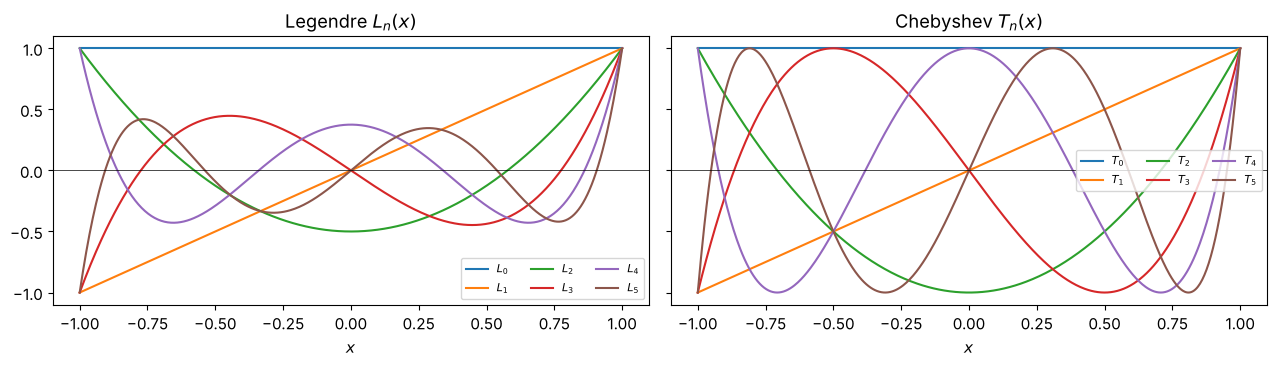
In 1D, the Legendre polynomials \(L_n\) are orthogonal with weight 1 on \([-1, 1]\). The Chebyshev polynomials \(T_n(\cos\theta) = \cos(n\theta)\) oscillate with equal amplitude everywhere (which makes them the best choice for minimizing the maximum error), but they are orthogonal only with the weight \(1/\sqrt{1 - x^2}\), which crowds them towards the edges.

x1 = np.linspace(-1, 1, 500)
fig, axes = plt.subplots(1, 2, figsize=(13, 3.8), sharey=True)
for n in range(6):
    axes[0].plot(x1, np.polynomial.legendre.Legendre.basis(n)(x1), label=f"$L_{n}$")
    axes[1].plot(x1, np.polynomial.chebyshev.Chebyshev.basis(n)(x1), label=f"$T_{n}$")
axes[0].set_title("Legendre $L_n(x)$"); axes[1].set_title("Chebyshev $T_n(x)$")
for ax in axes:
    ax.axhline(0, color="k", lw=0.5); ax.set_xlabel("$x$"); ax.legend(fontsize=8, ncol=3)
fig.tight_layout()

# a "midpoint" grid that does not contain x = ±1, where the Chebyshev weight diverges
Nq = 200
xq = np.linspace(-1, 1, Nq, endpoint=False) + 1/Nq
L = LegendrePolynomials(xq, xq)
T = ChebyshevPolynomials(xq, xq)
mask_q = L.mask.astype(bool)
ext_q = (-1, 1, -1, 1)

fig, axes = plt.subplots(2, 10, figsize=(16, 4.4))
for j in range(10):
    n, m = L.single_index_to_n_m(j)
    show(axes[0, j], L.eval_single(j), mask_q, ext_q, f"$L_{n}(x)L_{m}(y)$\n$j={j}$")
    show(axes[1, j], T.eval_single(j), mask_q, ext_q, f"$T_{n}(x)T_{m}(y)$")
fig.suptitle("Legendre (top) and Chebyshev (bottom) product bases up to order 3", y=1.02)
fig.tight_layout()

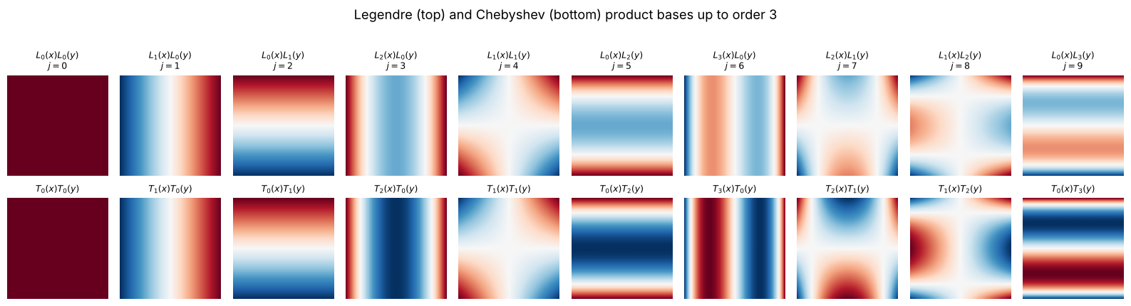
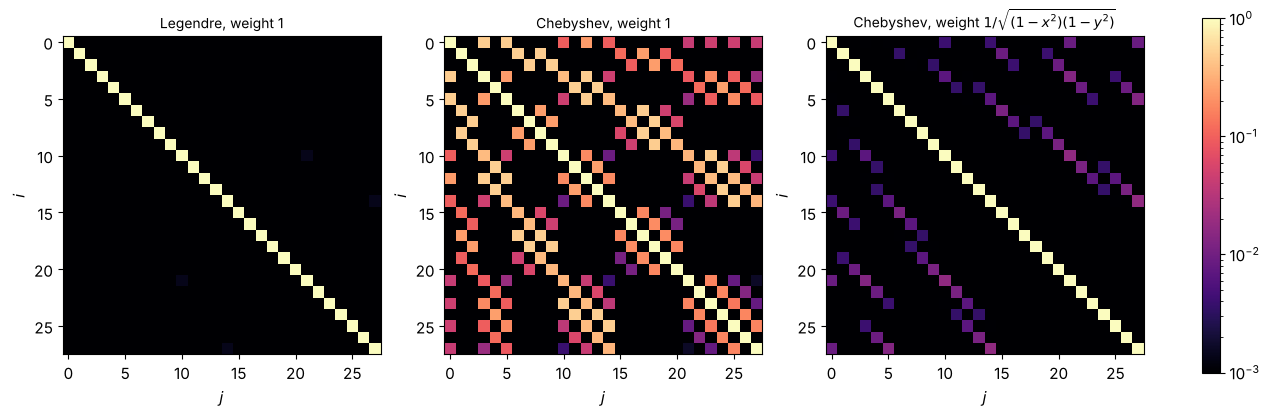
The Gram matrices of the first 28 functions (up to order 6) show the different notions of orthogonality: Legendre is orthogonal in the plain scalar product, Chebyshev is not, but becomes orthogonal with the weight \(w(x, y) = 1/\sqrt{(1 - x^2)(1 - y^2)}\). The functions of the two families only overlap with others of the same parity in \(x\) and in \(y\), hence the checkerboard pattern.

The Chebyshev weight diverges at the edges, which makes it hard to integrate on a uniform grid. We therefore use the weight averaged over each pixel, \(\frac{1}{\Delta x}\int_\text{pixel} \frac{dx}{\sqrt{1-x^2}} = \frac{\arcsin x_\text{right} - \arcsin x_\text{left}}{\Delta x}\); even so, the off-diagonal elements only drop to the percent level on this grid, compared with up to 90 % without the weight.

J28 = range(poly_basis_size(6))
QX, QY = np.meshgrid(xq, xq)
edges = np.linspace(-1, 1, Nq + 1)
w1 = np.diff(np.arcsin(edges))/np.diff(edges)   # pixel-averaged 1/sqrt(1 - x^2)
w_cheb = np.outer(w1, w1)
cases = (("Legendre, weight 1", [L.eval_single(j) for j in J28], 1.0),
         ("Chebyshev, weight 1", [T.eval_single(j) for j in J28], 1.0),
         ("Chebyshev, weight $1/\\sqrt{(1-x^2)(1-y^2)}$", [T.eval_single(j) for j in J28], w_cheb))
fig, axes = plt.subplots(1, 3, figsize=(15, 4.6))
for ax, (title, funcs, w) in zip(axes, cases):
    C = correlation(gram(funcs, xq, xq, w))
    im = ax.imshow(C, cmap="magma", norm=plt.matplotlib.colors.LogNorm(1e-3, 1), origin="upper")
    ax.set_title(title, fontsize=10); ax.set_xlabel("$j$"); ax.set_ylabel("$i$")
fig.colorbar(im, ax=axes, fraction=0.02)

<matplotlib.colorbar.Colorbar at 0x7fa89a985a90>

The analytic norm of the Legendre product functions is \(\langle L_n L_m | L_n L_m \rangle = \frac{2a}{2n+1}\frac{2b}{2m+1}\) (normalization_factor()). On this grid it is reproduced to a relative accuracy of:

num = np.diag(gram([L.eval_single(j) for j in J28], xq, xq))
ana = np.array([L.normalization_factor(j) for j in J28])
print(f"max |numeric/analytic - 1| for j < 28: {np.max(np.abs(num/ana - 1)):.1e}")
print(f"same via utils.scalar_product for j = 7: "
      f"{scalar_product(L.eval_single(7), L.eval_single(7), xq, xq)/L.normalization_factor(7) - 1:.1e}")

max |numeric/analytic - 1| for j < 28: 2.3e-03
same via utils.scalar_product for j = 7: -1.5e-04

5. Why orthogonality on the actual aperture matters

A popular shortcut is to describe the wavefront on a square aperture with Zernikes defined on the circumscribed circle (\(R = \sqrt 2\)). This works, but the Zernikes are not orthogonal on the square. As a consequence, a coefficient changes every time terms are added to the fit: “the amount of defocus” depends on how many other terms were fitted. With an orthogonal basis on the square (Legendre), the coefficients stay put.

We fit the same smooth function on the square with an increasing number of terms and follow two coefficients of each basis.

W_sq = np.exp(-((QX - 0.3)**2 + (QY + 0.25)**2)/(2*0.5**2)) + 0.3*np.cos(2*QX + QY)
Zsq = FringeZernikes(xq, xq, R_norm=np.sqrt(2))   # circle circumscribes the square

J_zern = np.arange(9, 50)
c_zern = np.array([Zsq.coeffs_from_field(W_sq, np.arange(1, J + 1))[[3, 8]] for J in J_zern])  # Z4, Z9
J_leg = np.arange(6, 50)
c_leg = np.array([L.coeffs_from_field(W_sq, np.arange(J))[[3, 5]] for J in J_leg])  # L2(x), L2(y)

fig, axes = plt.subplots(1, 3, figsize=(15, 4.2), gridspec_kw={"width_ratios": [1, 1.5, 1.5]})
show(axes[0], W_sq, mask_q, ext_q, "wavefront on the square")
axes[0].add_patch(plt.Circle((0, 0), np.sqrt(2), fill=False, ls="--"))
axes[0].set_xlim(-1.45, 1.45); axes[0].set_ylim(-1.45, 1.45)
axes[1].plot(J_zern, c_zern[:, 0], ".-", label="$c_4$ (defocus)")
axes[1].plot(J_zern, c_zern[:, 1], ".-", label="$c_9$ (spherical)")
axes[1].set_title("Zernikes on the circumscribed circle"); axes[1].set_xlabel("number of fitted terms")
axes[2].plot(J_leg, c_leg[:, 0], ".-", label="$c_3$ ($L_2(x)$)")
axes[2].plot(J_leg, c_leg[:, 1], ".-", label="$c_5$ ($L_2(y)$)")
axes[2].set_title("Legendre on the square"); axes[2].set_xlabel("number of fitted terms")
for ax in axes[1:]:
    ax.set_ylabel("coefficient"); ax.legend()
fig.tight_layout()

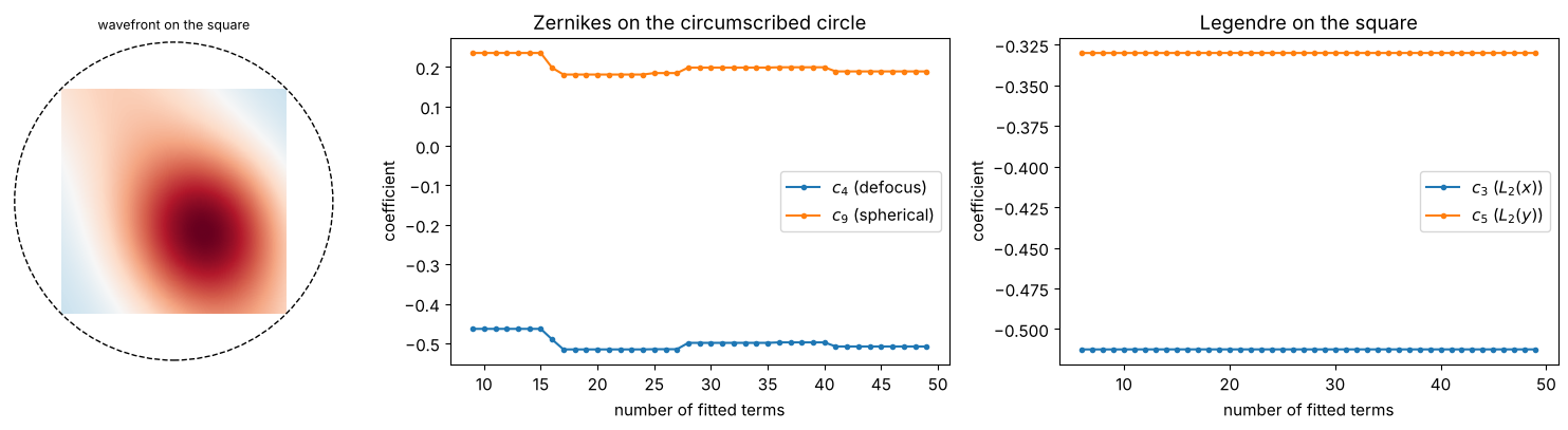
The Zernike coefficients jump whenever a function with a strong projection onto defocus or spherical aberration enters the fit; the Legendre coefficients converge to their final values almost immediately and then only change at the level of the discretization error.

6. Arbitrary apertures: numerical orthogonalization

Telescopes have a central obscuration, segmented mirrors are hexagonal. On such apertures the Zernikes lose their orthogonality as well. On an annulus with obscuration ratio \(\varepsilon = 0.5\), for example, defocus \(Z_4 = 2\rho^2 - 1\) no longer averages to zero, so it overlaps with piston.

NumericallyOrthogonalized samples a basis, restricts it to a new mask and runs a Gram-Schmidt procedure (via a QR decomposition) on the grid. The resulting functions are exactly orthogonal on that grid and keep their original norms (or take the norms given by norm_func).

xa = grid1d(-1.02, 1.02, 201)
eps = 0.5
ann = annular_mask(xa, xa, 1.0, eps)
mask_a = ann.astype(bool)
ext_a = (xa[0], xa[-1], xa[0], xa[-1])
J16 = np.arange(1, 17)

Za = FringeZernikes(xa, xa)
Za_orth = NumericallyOrthogonalized(xa, xa, FringeZernikes, J16, new_mask=ann)

G_plain = gram([Za.eval_single(j)*ann for j in J16], xa, xa)
G_orth = gram([Za_orth.eval_single(j) for j in J16], xa, xa)

fig, axes = plt.subplots(1, 2, figsize=(11, 4.6))
for ax, G_, title in zip(axes, (G_plain, G_orth), ("Fringe Zernikes on the annulus", "numerically orthogonalized")):
    im = ax.imshow((correlation(G_)), cmap="magma", norm=plt.matplotlib.colors.LogNorm(1e-4, 1),
                   extent=(0.5, 16.5, 16.5, 0.5), origin="upper")
    ax.set_title(title); ax.set_xlabel("$j$"); ax.set_ylabel("$i$")
    ax.set_xticks([1, 4, 8, 12, 16]); ax.set_yticks([1, 4, 8, 12, 16])
fig.colorbar(im, ax=axes, fraction=0.03)

<matplotlib.colorbar.Colorbar at 0x7fa89a4334d0>

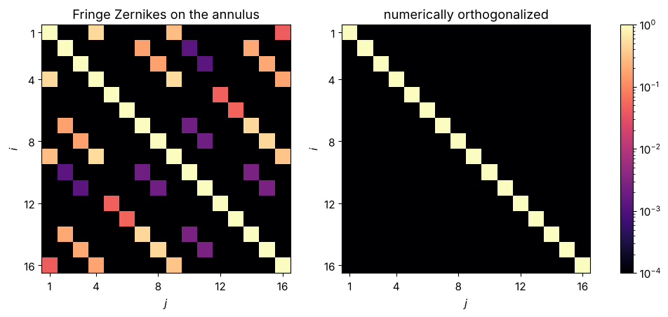
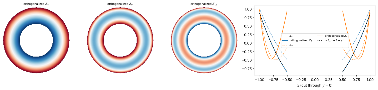
The orthogonalized functions are the (numerical) annular Zernike polynomials. For defocus, Gram-Schmidt only has to remove the mean over the annulus: since \(\langle \rho^2 \rangle = (1 + \varepsilon^2)/2\) there, the result must be proportional to \(2\rho^2 - 1 - \varepsilon^2\), which is the analytic annular defocus. Higher orders change more, e.g. spherical aberration, which has to be made orthogonal to both piston and defocus.

row = len(xa)//2
fig, axes = plt.subplots(1, 4, figsize=(16, 3.8), gridspec_kw={"width_ratios": [1, 1, 1, 1.8]})
for ax, j in zip(axes[:2], (4, 9)):
    show(ax, Za_orth.eval_single(j), mask_a, ext_a, f"orthogonalized $Z_{{{j}}}$")
show(axes[2], Za_orth.eval_single(16), mask_a, ext_a, "orthogonalized $Z_{16}$")
r = xa[mask_a[row]]
for j, col in ((4, "C0"), (9, "C1")):
    axes[3].plot(xa, np.where(mask_a[row], Za.eval_single(j)[row], np.nan), "--", color=col, lw=1,
                 label=f"$Z_{{{j}}}$")
    axes[3].plot(xa, np.where(mask_a[row], Za_orth.eval_single(j)[row], np.nan), color=col,
                 label=f"orthogonalized $Z_{{{j}}}$")
ref = 2*xa**2 - 1 - eps**2
scale = np.sum(Za_orth.eval_single(4)[row][mask_a[row]]*ref[mask_a[row]])/np.sum(ref[mask_a[row]]**2)
axes[3].plot(xa, np.where(mask_a[row], scale*ref, np.nan), "k:", lw=2, label="$\\propto 2\\rho^2 - 1 - \\varepsilon^2$")
axes[3].set_xlabel("$x$ (cut through $y = 0$)"); axes[3].legend(fontsize=8, ncol=2)
fig.tight_layout()

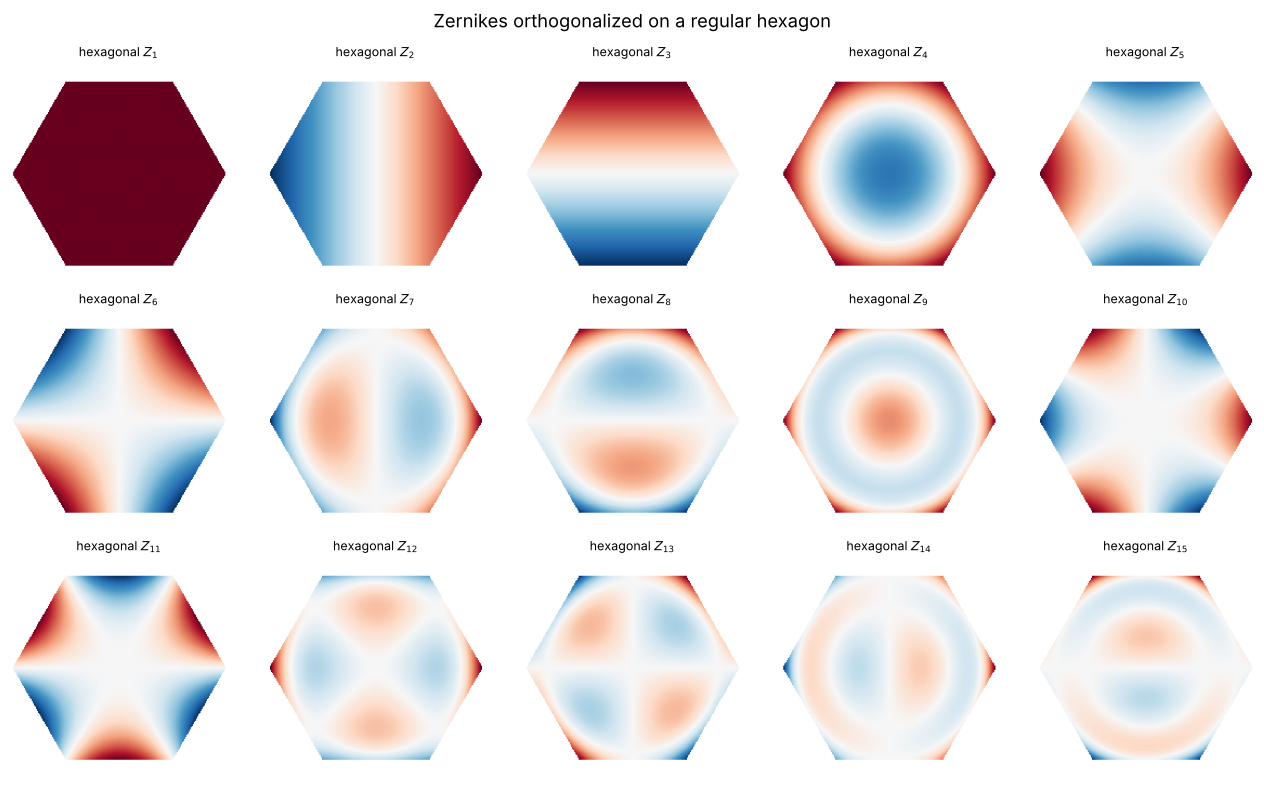
A hexagonal aperture works the same way: any mask, e.g. from mask_from_polygon(), can be used.

phi_hex = np.linspace(0, 2*np.pi, 7)
hexagon = mask_from_polygon(xa, xa, np.cos(phi_hex), np.sin(phi_hex))
mask_h = hexagon.astype(bool)
J15 = np.arange(1, 16)
Zh_orth = NumericallyOrthogonalized(xa, xa, FringeZernikes, J15, new_mask=hexagon)

fig, axes = plt.subplots(3, 5, figsize=(13, 8))
for ax, j in zip(axes.flat, J15):
    show(ax, Zh_orth.eval_single(j), mask_h, ext_a, f"hexagonal $Z_{{{j}}}$")
fig.suptitle("Zernikes orthogonalized on a regular hexagon")
fig.tight_layout()

Again the coefficients tell the story. We fit a wavefront on the annulus with the plain Zernikes (restricted to the annulus) and with the orthogonalized set, and follow the piston and defocus coefficients. With plain Zernikes, “piston” is not the mean of the wavefront and changes with the number of terms; with the orthogonalized basis it is the mean, independent of \(J\).

XA, YA = np.meshgrid(xa, xa)
W_a = (0.6*(2*(XA**2 + YA**2) - 1) + 0.3*np.exp(-((XA + 0.5)**2 + (YA - 0.4)**2)/0.1))*ann
J36a = np.arange(1, 37)
Za_orth36 = NumericallyOrthogonalized(xa, xa, FringeZernikes, J36a, new_mask=ann)

def masked_lstsq(basis, inds, field, mask):
    M = np.array([basis.eval_single(j)[mask] for j in inds]).T
    return np.linalg.lstsq(M, field[mask], rcond=None)[0]

Jfit = np.arange(4, 37)
c_plain = np.array([masked_lstsq(Za, np.arange(1, J + 1), W_a, mask_a)[[0, 3]] for J in Jfit])
c_orth = np.array([Za_orth36.coeffs_from_field(W_a, np.arange(1, J + 1))[[0, 3]] for J in Jfit])

fig, axes = plt.subplots(1, 3, figsize=(15, 4), gridspec_kw={"width_ratios": [1, 1.5, 1.5]})
show(axes[0], W_a, mask_a, ext_a, "wavefront on the annulus")
for ax, c, title in ((axes[1], c_plain, "plain Zernikes"), (axes[2], c_orth, "orthogonalized")):
    ax.plot(Jfit, c[:, 0], ".-", label="$c_1$ (piston)")
    ax.plot(Jfit, c[:, 1], ".-", label="$c_4$ (defocus)")
    ax.axhline(W_a[mask_a].mean(), color="k", lw=0.8, ls=":", label="mean of $W$")
    ax.set_title(title); ax.set_xlabel("number of fitted terms"); ax.set_ylabel("coefficient")
    ax.legend(fontsize=9)
fig.tight_layout()

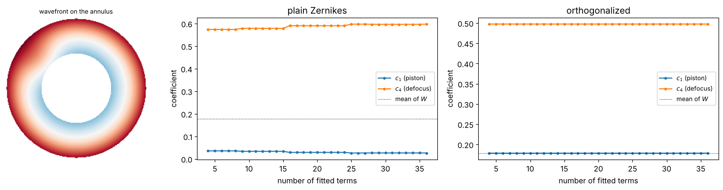
Note that masked_lstsq() above is needed for the plain Zernikes: FringeZernikes are non-zero in the central hole, and coeffs_from_field() fits on the whole grid. The orthogonalized functions vanish outside their new mask, so the built-in fit works directly.

7. Rescaling: coefficients as peak values

With the Fringe normalization, a coefficient \(c_j\) is the peak value of the term on the unit circle. On a smaller or non-circular aperture this is no longer true: on the hexagon inscribed in the unit circle, most Zernikes never reach \(|Z_j| = 1\). RescaledBasis wraps a basis, applies a new mask and rescales every function with scale_val_func(j)/scale_func(B_j). With scale_func = max |B_j| and scale_val_func = 1, each coefficient is again the peak deviation on the aperture.

Zh_rescaled = RescaledBasis(xa, xa, FringeZernikes, mask=hexagon,
                            scale_func=lambda v: np.max(np.abs(v)), scale_val_func=lambda j: 1.0)
peak_plain = [np.max(np.abs(Za.eval_single(j)*hexagon)) for j in J15]
with contextlib.redirect_stdout(io.StringIO()):   # RescaledBasis prints every factor
    peak_rescaled = [np.max(np.abs(Zh_rescaled.eval_single(j))) for j in J15]
    Z7_hex = Zh_rescaled.eval_single(7)
print("max |Z_j| of the rescaled functions:", np.round(peak_rescaled, 3))

fig, axes = plt.subplots(1, 2, figsize=(13, 4), gridspec_kw={"width_ratios": [2.2, 1]})
axes[0].bar(J15, peak_plain)
axes[0].set_xticks(J15); axes[0].set_xlabel("Fringe index $j$"); axes[0].set_ylabel("max $|Z_j|$ on the hexagon")
axes[0].set_title("Peak value of the plain Zernikes on the inscribed hexagon")
show(axes[1], Z7_hex, mask_h, ext_a, f"rescaled $Z_7$: max = {np.max(np.abs(Z7_hex)):.2f}", vmax=1)
fig.tight_layout()

max |Z_j| of the rescaled functions: [1. 1. 1. 1. 1. 1. 1. 1. 1. 1. 1. 1. 1. 1. 1.]

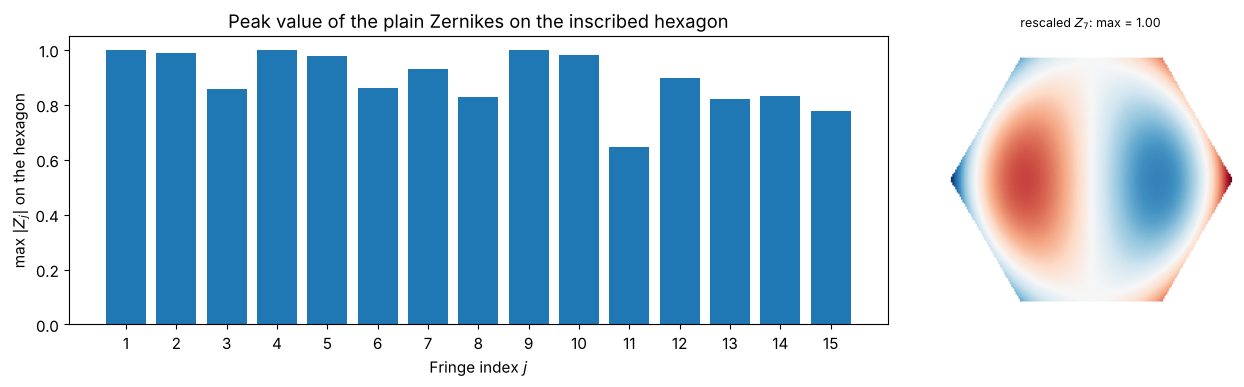
Functions that peak at the rim in the direction of a vertex (piston, \(x\) tilt, defocus, spherical aberration) still reach 1. The others lose amplitude: \(y\) tilt peaks at the top edge, \(\sqrt 3/2 \approx 0.87\), and the trefoil \(Z_{11}\), whose maxima point at the edge midpoints, reaches only \((\sqrt 3/2)^3 \approx 0.65\). After rescaling, all of them have a peak value of exactly 1.

8. Scattered data

Measurements do not always come on a grid: a coordinate measuring machine probes a surface at a few hundred points, a Shack-Hartmann sensor at its lenslet positions. coeffs_from_scattered() fits the coefficients directly to such data, and B(indices, coeffs) then gives the result on any grid. We simulate 120 noisy measurements of a wavefront built from 15 Zernikes.

rng = np.random.default_rng(1)
J15_true = np.arange(1, 16)
c_true = rng.normal(0, 0.3, 15)/np.sqrt(J15_true)
noise = 0.02

def sample_disk(n):
    r, phi = np.sqrt(rng.random(n)), 2*np.pi*rng.random(n)
    return r*np.cos(phi), r*np.sin(phi)

xs, ys = sample_disk(120)
data = Zg(J15_true, c_true, xs, ys) + rng.normal(0, noise, xs.shape)
c_fit = Zg.coeffs_from_scattered(xs, ys, data, J15_true)

W_true = Zg(J15_true, c_true)
W_rec = Zg(J15_true, c_fit)
vmax = np.max(np.abs(W_true[mask_g]))
fig, axes = plt.subplots(1, 4, figsize=(16, 4), gridspec_kw={"width_ratios": [1, 1, 1, 1.4]})
show(axes[0], W_true, mask_g, ext, "true wavefront", vmax)
axes[1].scatter(xs, ys, c=data, cmap="RdBu_r", vmin=-vmax, vmax=vmax, s=18)
axes[1].add_patch(plt.Circle((0, 0), 1, fill=False)); axes[1].set_aspect("equal"); axes[1].axis("off")
axes[1].set_title("120 noisy samples", fontsize=9)
show(axes[2], W_true - W_rec, mask_g, ext, f"error of the reconstruction (×10)\nrms = {rms(W_true - W_rec, mask_g):.4f}", vmax/10)
axes[3].bar(J15_true - 0.2, c_true, 0.4, label="true")
axes[3].bar(J15_true + 0.2, c_fit, 0.4, label="fitted")
axes[3].set_xticks(J15_true); axes[3].set_xlabel("Fringe index"); axes[3].legend()
fig.tight_layout()

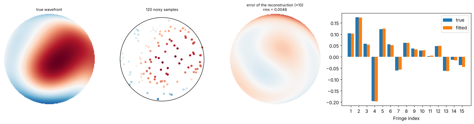
How many samples are needed? The fit has as many unknowns as terms. With too few points the problem is badly conditioned and the noise is amplified enormously; with many points the error decreases like \(1/\sqrt{N_\text{points}}\), as for any averaging of noise. The same 15-term wavefront is fitted with \(J = 15\) and with \(J = 36\) terms (the extra 21 coefficients should come out as zero).

n_pts = np.unique(np.round(np.logspace(np.log10(12), np.log10(3000), 22)).astype(int))
curves = {}
for J in (15, 36):
    inds = np.arange(1, J + 1)
    errs = []
    for n in n_pts:
        e = []
        for trial in range(20):
            xs_, ys_ = sample_disk(n)
            d = Zg(J15_true, c_true, xs_, ys_) + rng.normal(0, noise, n)
            if n < J:
                e.append(np.nan); continue
            c = Zg.coeffs_from_scattered(xs_, ys_, d, inds)
            e.append(rms(W_true - Zg(inds, c), mask_g))
        errs.append(np.nanmedian(e) if np.isfinite(e).any() else np.nan)
    curves[J] = np.array(errs)

fig, ax = plt.subplots(figsize=(7.5, 4.5))
for J, e in curves.items():
    ax.loglog(n_pts, e, "o-", label=f"$J = {J}$ fitted terms")
    ax.axvline(J, color=ax.lines[-1].get_color(), ls=":", lw=1)
ax.loglog(n_pts, noise*np.sqrt(15/n_pts), "k--", lw=1, label="$\\sigma\\sqrt{J/N}$, $J = 15$")
ax.set_xlabel("number of sample points $N$"); ax.set_ylabel("rms reconstruction error (median of 20)")
ax.set_title(f"Fit to scattered data, noise σ = {noise}"); ax.legend()
fig.tight_layout()

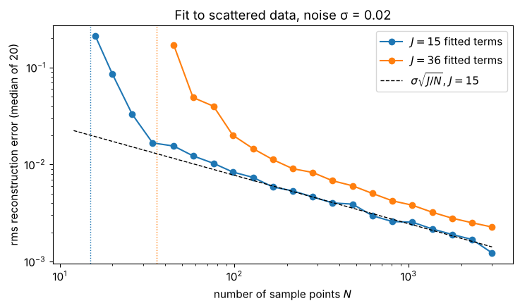
Close to \(N = J\) (dotted lines) the error explodes; a few times more points than terms are needed before the fit is limited by the noise alone. Fitting more terms than the wavefront contains costs accuracy at a given \(N\), because the extra coefficients fit the noise.

9. Presampling for speed

Every eval_single() call recomputes the polynomial on the grid. In iterative algorithms (fits in a loop, optimization over coefficients) it pays to sample the needed functions once: PresampledBasisSet wraps any basis and replaces the evaluation by a dictionary lookup, while passing through the mask and norms.

xb = grid1d(-1, 1, 512)
inds = np.arange(1, 37)
Z_live = FringeZernikes(xb, xb)
Z_pre = PresampledBasisSet(xb, xb, FringeZernikes, inds)
coeffs = rng.normal(size=36)

for name, B in (("FringeZernikes", Z_live), ("PresampledBasisSet", Z_pre)):
    t0 = time.perf_counter()
    for _ in range(5):
        B(inds, coeffs)
    print(f"{name:20s}: {(time.perf_counter() - t0)/5*1e3:6.1f} ms per evaluation of 36 terms on 512 × 512")
print("identical results:", np.allclose(Z_live(inds, coeffs), Z_pre(inds, coeffs)))

FringeZernikes      :  298.2 ms per evaluation of 36 terms on 512 × 512
PresampledBasisSet  :   38.3 ms per evaluation of 36 terms on 512 × 512

identical results: True

Summary

• Zernikes, Legendre and Chebyshev polynomials are orthogonal on their own aperture (disk or rectangle), Chebyshev only with its weight function. On a grid, orthogonality holds up to a discretization error \(\propto 1/N\) from the aperture edge.

• Least-squares fitting ("LSTSQ") is the robust default; overlap integrals ("DI") only work as well as the discrete orthogonality.

• On any other aperture (square, annulus, hexagon), a basis that is not orthogonal there gives coefficients that depend on which other terms are fitted. NumericallyOrthogonalized fixes that for an arbitrary mask; RescaledBasis restores the meaning of a coefficient as a peak value.

• Scattered data can be fitted directly, with a few times more points than terms.

The classes Polynomials (plain monomials) and the function basis_from_generating_function() exist in the module but are not implemented yet.

References

• F. Zernike, “Beugungstheorie des Schneidenverfahrens und seiner verbesserten Form, der Phasenkontrastmethode”, Physica 1, 689-704 (1934).

• R. J. Noll, “Zernike polynomials and atmospheric turbulence”, J. Opt. Soc. Am. 66, 207-211 (1976).

• J. C. Wyant and K. Creath, “Basic wavefront aberration theory for optical metrology”, in R. R. Shannon and J. C. Wyant (eds.), Applied Optics and Optical Engineering, Vol. XI, Academic Press (1992).

• V. N. Mahajan and G.-m. Dai, “Orthonormal polynomials in wavefront analysis: analytical solution”, J. Opt. Soc. Am. A 24, 2994-3016 (2007).

• M. Born and E. Wolf, Principles of Optics, 7th ed., Cambridge University Press (1999).