Chirp-z transform: zoomed spectra, shifted and scaled propagation

An FFT evaluates a Fourier sum on one fixed grid: \(N\) frequencies with the spacing \(2\pi/L\). Often only a small part of that grid is of interest, but with a finer sampling: the core of a PSF, one diffraction order, an off-axis detector. Zero padding gets there at the cost of huge arrays. The chirp-z transform (Bluestein 1970) evaluates

\[ X_m = \sum_{n=0}^{N-1} x_n\, a^{-n} w^{nm}, \qquad m = 0, \dots, M-1, \]

for any start \(a\) and step \(w\) with three FFTs of length \(\geq N + M - 1\). With \(a = e^{i k_0 \Delta x}\), \(w = e^{-i \Delta k \Delta x}\) it is a Fourier sum on the frequencies \(k_0 + m\,\Delta k\) with free \(k_0\), \(\Delta k\) and \(M\).

Function	What it does
fft.czt(x, M, w, a)	Bluestein’s chirp-z transform (any axis)
fft.zoom_FT(f, x, y, kx_out, ky_out)	FT() on any equidistant frequency grid
fft.zoom_inv_FT(F, kx, ky, x_out, y_out)	inv_FT() on any equidistant grid of positions
propagators.shifted_angular_spectrum()	exact propagation onto an off-axis, rescaled window (Matsushima 2010)
propagators.fresnel_scaled()	Fresnel integral onto any window
propagators.fraunhofer_scaled()	Fraunhofer integral onto any window
propagators.far_field()	far field amplitude in chosen directions
imaging.get_psf(..., x_out, y_out)	PSF on any window without padding

All of them keep the pyoptics conventions: fields vary as \(\exp(i(\mathbf{k}\cdot\mathbf{r} - \omega t))\), FT() has the kernel \(e^{-i\mathbf{k}\cdot\mathbf{r}}\) and returns plane wave amplitudes. Lengths are in units of the wavelength.

import time
import numpy as np
import matplotlib.pyplot as plt

from pyoptics.fft import FT, czt, zoom_FT, zoom_inv_FT
from pyoptics.utils import grid1d, frequencies, pad
from pyoptics.analytical import airy_pattern
from pyoptics.imaging import get_psf
from pyoptics.propagators import (rayleigh_sommerfeld_I_TF, shifted_angular_spectrum,
                                  fresnel_scaled, fresnel_rescaling, far_field)

plt.rcParams.update({"figure.dpi": 100, "image.origin": "lower", "font.size": 11})
WL = 1.0
K = 2*np.pi/WL

1. The chirp-z transform is a DFT on any frequency grid

First a check against the definition: for \(a = 1\), \(w = e^{-2\pi i/N}\), \(M = N\) the chirp-z transform is the DFT, and for any other \(a\), \(w\) it equals the direct sum (here for a random signal; the error is round-off).

rng = np.random.default_rng(0)
x = rng.normal(size=300) + 1j*rng.normal(size=300)
X_fft = np.fft.fft(x)
print("czt vs. np.fft.fft:  max relative error {:.1e}".format(np.abs(czt(x) - X_fft).max()/np.abs(X_fft).max()))

M, w, a = 400, np.exp(-0.0071j), np.exp(0.83j)
n, m = np.arange(len(x)), np.arange(M)
direct = (x[None, :]*a**(-n[None, :])*w**(n[None, :]*m[:, None])).sum(axis=1)
print("czt vs. direct sum: max relative error {:.1e}".format(np.abs(czt(x, M, w, a) - direct).max()/np.abs(direct).max()))

czt vs. np.fft.fft:  max relative error 5.5e-13
czt vs. direct sum: max relative error 4.1e-14

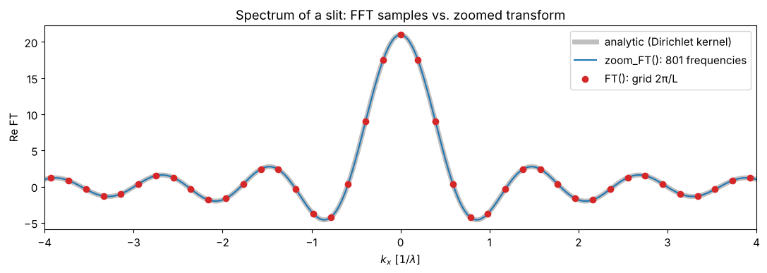
zoom_FT() uses this to evaluate the spectrum of a field on a frequency grid of our choice. The example is a 1D slit of width \(10\lambda\) sampled on \(N = 64\) points: the FFT gives the spectrum only at the multiples of \(2\pi/L\) (dots); zoom_FT() gives it on a 20× finer grid over the central lobes (line), which is the same as the FFT of the 20× zero padded field, but uses arrays of length \(\approx N + M\) instead of \(20N\). The analytic spectrum of the sampled slit (a Dirichlet kernel) lies on top.

L, N = 32.0, 64
x = grid1d(-L/2, L/2, N)
f = (np.abs(x) <= 5.0).astype(complex)[None, :]          # 1 x N "image"
kx = frequencies(x)

kx_fine = np.linspace(-4, 4, 801)
F_zoom = zoom_FT(f, x, np.array([0.0]), kx_fine, np.array([0.0]))[0]
F_fft = FT(f)[0]

dx = x[1] - x[0]
n_open = np.count_nonzero(np.abs(x) <= 5.0)                 # 21 open samples, centered
with np.errstate(invalid="ignore", divide="ignore"):
    dirichlet = np.where(np.isclose(np.sin(kx_fine*dx/2), 0), n_open,
                         np.sin(n_open*kx_fine*dx/2)/np.sin(kx_fine*dx/2))

fig, ax = plt.subplots(figsize=(11, 4))
ax.plot(kx_fine, dirichlet, color="0.75", lw=5, label="analytic (Dirichlet kernel)")
ax.plot(kx_fine, F_zoom.real, "C0", lw=1.5, label="zoom_FT(): 801 frequencies")
ax.plot(kx, F_fft.real, "o", color="C3", ms=6, label="FT(): grid 2π/L")
ax.set_xlim(-4, 4)
ax.set_xlabel(r"$k_x\ [1/\lambda]$"); ax.set_ylabel("Re FT")
ax.legend(); ax.set_title("Spectrum of a slit: FFT samples vs. zoomed transform")
plt.tight_layout()
print("max deviation from the analytic sum: {:.1e}".format(np.abs(F_zoom - dirichlet).max()))

max deviation from the analytic sum: 9.0e-13

How much does zooming save? The table compares zoom_FT() onto a \(256^2\) window with the zero-padded FFT that gives the same frequency spacing (zoom factor \(Z\): the padded field has \((ZN)^2\) samples, of which we only need a small part).

N = 256
x = grid1d(-64, 64, N)
X, Y = np.meshgrid(x, x)
f = np.exp(-(X**2 + Y**2)/10.0**2).astype(complex)
dk = 2*np.pi/(x[-1] - x[0] + x[1] - x[0])
print(" zoom    padded FFT [s]   zoom_FT [s]   max difference")
for Z in (4, 8, 16):
    t0 = time.perf_counter()
    f_pad, x_pad, _ = pad(f, x, x, factor=Z)
    F_pad = FT(f_pad)
    k_pad = frequencies(x_pad)
    t_pad = time.perf_counter() - t0
    sl = slice(Z*N//2 - 128, Z*N//2 + 128)
    t0 = time.perf_counter()
    F_zoom = zoom_FT(f, x, x, k_pad[sl], k_pad[sl])
    t_zoom = time.perf_counter() - t0
    print("{:4d}    {:12.3f}   {:10.3f}     {:.1e}".format(Z, t_pad, t_zoom, np.abs(F_zoom - F_pad[sl, sl]).max()/np.abs(F_pad).max()))

 zoom    padded FFT [s]   zoom_FT [s]   max difference

   4           0.301        0.012     1.1e-12

   8           0.971        0.011     6.5e-13

  16           3.979        0.009     1.0e-12

2. Zooming into the PSF

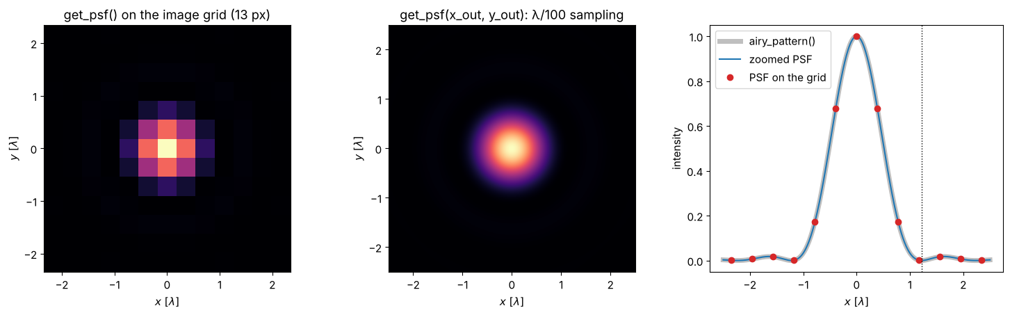
imaging.get_psf() samples the pupil on the frequency grid of the image plane grid x, y; the image grid therefore has to be large to sample the pupil well, and fine to resolve the PSF – usually conflicting wishes. With x_out, y_out the PSF is evaluated by a chirp-z transform of the pupil on any window: x, y only set the pupil sampling.

Here the image grid has \(256^2\) points with \(\Delta x = 0.39\lambda\) (a pupil radius of 50 samples at NA 0.5); the zoomed PSF is evaluated on a \(\lambda/100\) grid over the Airy disk. Its cut agrees with the analytic Airy pattern to the accuracy of the pupil sampling.

NA = 0.5
L, N = 100*WL, 256
x = grid1d(-L/2, L/2, N)
x_out = np.linspace(-2.5, 2.5, 501)

psf_grid = get_psf(x, x, NA, K)
psf_zoom = get_psf(x, x, NA, K, x_out=x_out, y_out=x_out)

fig, axes = plt.subplots(1, 3, figsize=(15, 4.6))
ext = [x[0], x[-1], x[0], x[-1]]
sel = np.abs(x) <= 2.5
axes[0].imshow(np.abs(psf_grid[np.ix_(sel, sel)])**2, extent=[x[sel][0], x[sel][-1]]*2, cmap="magma")
axes[0].set_title("get_psf() on the image grid ({} px)".format(np.count_nonzero(sel)))
axes[1].imshow(np.abs(psf_zoom)**2, extent=[x_out[0], x_out[-1]]*2, cmap="magma")
axes[1].set_title("get_psf(x_out, y_out): λ/100 sampling")
for ax in axes[:2]:
    ax.set_xlabel(r"$x\ [\lambda]$"); ax.set_ylabel(r"$y\ [\lambda]$")

I_cut = np.abs(psf_zoom[250])**2
axes[2].plot(x_out, airy_pattern(np.abs(x_out), NA, WL), color="0.75", lw=5, label="airy_pattern()")
axes[2].plot(x_out, I_cut, "C0", label="zoomed PSF")
axes[2].plot(x[sel], np.abs(psf_grid[N//2, sel])**2, "o", color="C3", label="PSF on the grid")
axes[2].axvline(0.61*WL/NA, color="k", ls=":", lw=1)
axes[2].set_xlabel(r"$x\ [\lambda]$"); axes[2].set_ylabel("intensity")
axes[2].legend()
plt.tight_layout()
print("max deviation from Airy: {:.1e}".format(np.abs(I_cut - airy_pattern(np.abs(x_out), NA, WL)).max()))

max deviation from Airy: 4.3e-04

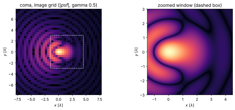
The output window can be placed anywhere, e.g. on the comatic flare of an aberrated PSF. The PSF of the discrete pupil is periodic with the image window \(L\); within it, every window is exact.

coma = lambda P_x, P_y: 2*np.pi*0.4*(3*(P_x**2 + P_y**2) - 2)*P_x   # 0.4 waves Fringe Z7
psf_coma = get_psf(x, x, NA, K, phase=coma)
x_win, y_win = np.linspace(-1.5, 4.5, 301), np.linspace(-3, 3, 301)
psf_win = get_psf(x, x, NA, K, phase=coma, x_out=x_win, y_out=y_win)

fig, axes = plt.subplots(1, 2, figsize=(11, 4.6))
sel = np.abs(x) <= 8
axes[0].imshow(np.abs(psf_coma[np.ix_(sel, sel)])**0.5, extent=[x[sel][0], x[sel][-1]]*2, cmap="magma")
axes[0].add_patch(plt.Rectangle((x_win[0], y_win[0]), 6, 6, fill=False, ec="w", ls="--"))
axes[0].set_title(r"coma, image grid ($|psf|$, gamma 0.5)")
axes[1].imshow(np.abs(psf_win)**0.5, extent=[x_win[0], x_win[-1], y_win[0], y_win[-1]], cmap="magma")
axes[1].set_title("zoomed window (dashed box)")
for ax in axes:
    ax.set_xlabel(r"$x\ [\lambda]$"); ax.set_ylabel(r"$y\ [\lambda]$")
plt.tight_layout()
print("Strehl ratio from the zoomed PSF (peak value): {:.3f}".format(np.max(np.abs(psf_win))**2))

Strehl ratio from the zoomed PSF (peak value): 0.446

3. The focus of a lens with fresnel_scaled()

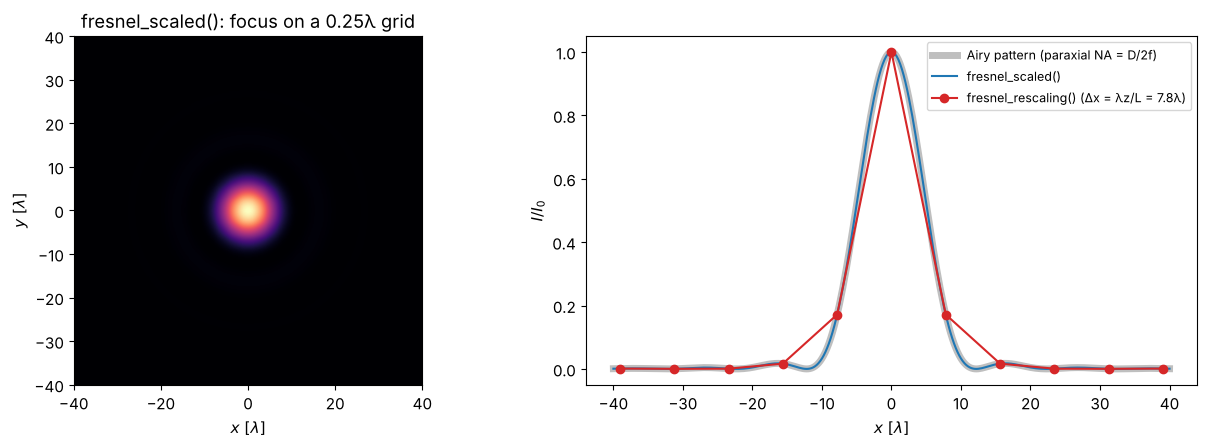
fresnel_scaled() evaluates the single-transform Fresnel integral

\[ U(x, y) = \frac{e^{ikz}}{i\lambda z} e^{ik(x^2+y^2)/2z} \iint U'(x', y')\, e^{ik(x'^2+y'^2)/2z}\, e^{-ik(xx' + yy')/z}\,dx'\,dy' \]

with zoom_FT() at \(k_x = kx/z\). fresnel_rescaling() evaluates the same integral by FFT, but its output spacing is fixed to \(\lambda z/L\) – at the focus of a lens usually far too coarse. Here a lens with \(f = 2000\lambda\) and an aperture of \(D = 200\lambda\) (\(\mathrm{NA} \approx 0.05\), Airy radius \(12\lambda\)) is sampled with \(512^2\) points; fresnel_rescaling() puts only about 2 samples into the Airy disk.

f_lens, D = 2000.0, 200.0
L, N = 256.0, 512
x = grid1d(-L/2, L/2, N)
X, Y = np.meshgrid(x, x)
pupil = (X**2 + Y**2 <= (D/2)**2)*np.exp(-1j*K*(X**2 + Y**2)/(2*f_lens))

U_resc, x_resc, y_resc = fresnel_rescaling(pupil, x, x, f_lens, WL)
x_out = np.linspace(-40, 40, 321)
U_zoom, _, _ = fresnel_scaled(pupil, x, x, f_lens, WL, x_out, x_out)

NA_lens = np.sin(np.arctan(D/2/f_lens))
I0 = np.abs(U_zoom[160, 160])**2
fig, axes = plt.subplots(1, 2, figsize=(13, 4.6))
axes[0].imshow(np.abs(U_zoom)**2/I0, extent=[x_out[0], x_out[-1]]*2, cmap="magma", vmax=1)
axes[0].set_title("fresnel_scaled(): focus on a 0.25λ grid")
axes[0].set_xlabel(r"$x\ [\lambda]$"); axes[0].set_ylabel(r"$y\ [\lambda]$")
sel = np.abs(x_resc) <= 40
axes[1].plot(x_out, airy_pattern(np.abs(x_out), D/2/f_lens, WL), color="0.75", lw=5, label="Airy pattern (paraxial NA = D/2f)")
axes[1].plot(x_out, np.abs(U_zoom[160])**2/I0, "C0", label="fresnel_scaled()")
axes[1].plot(x_resc[sel], np.abs(U_resc[N//2, sel])**2/I0, "o-", color="C3", label="fresnel_rescaling() (Δx = λz/L = {:.1f}λ)".format(x_resc[1] - x_resc[0]))
axes[1].set_xlabel(r"$x\ [\lambda]$"); axes[1].set_ylabel(r"$I/I_0$"); axes[1].legend(fontsize=9)
plt.tight_layout()
print("first zero: fresnel_scaled() {:.2f}λ, Airy 0.61λ/NA = {:.2f}λ".format(
    x_out[160 + np.argmin(np.abs(U_zoom[160, 160:240]))], 0.61*WL*2*f_lens/D))

first zero: fresnel_scaled() 12.25λ, Airy 0.61λ/NA = 12.20λ

Two sampling conditions remain, and fresnel_scaled() warns about both: the input chirp \(e^{ikr'^2/2z}\) must be sampled on the input grid (\(|z| \gtrsim 2\max|x'|\Delta x/\lambda\); above, the lens phase cancels most of it), and the result is periodic with \(\lambda z/\Delta x\), so the output window should be smaller than that. For short distances the angular spectrum is the right tool.

4. Off-axis propagation with the shifted angular spectrum method

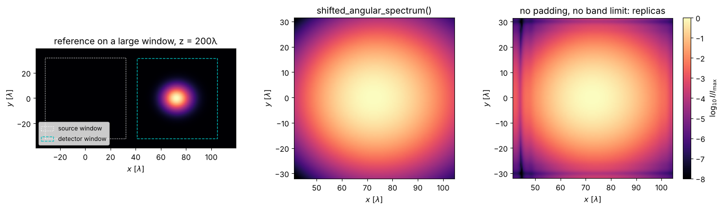
A Gaussian beam (\(w_0 = 5\lambda\)) is tilted by 20° and propagates by \(z = 200\lambda\): it arrives about \(73\lambda\) off axis, far outside the input window of \(64\lambda\). The ordinary angular spectrum method needs a window that holds both the source and the detector. shifted_angular_spectrum() evaluates

\[ U(x, y, z) = \frac{1}{N_xN_y}\sum_{mn} A_{mn}\, e^{i(k_x x + k_y y + k_z z)} \]

directly on the detector window with zoom_inv_FT(). The input is padded to the size of source plus detector window, and only plane waves that travel from the source window into the detector window are kept, i.e. the lateral shift \(z\,k_x/k_z\) lies between \(\min x_\mathrm{out} - \max x'\) and \(\max x_\mathrm{out} - \min x'\) (Matsushima’s band limit). The reference is an angular spectrum computation on a \(16\times\) larger window.

L, N, z, theta, w0 = 64.0, 128, 200.0, np.deg2rad(20), 5.0
x = grid1d(-L/2, L/2, N)
X, Y = np.meshgrid(x, x)
source = np.exp(-(X**2 + Y**2)/w0**2)*np.exp(1j*K*np.sin(theta)*X)

# reference: large window
N_ref = 2048
f_ref, x_ref, _ = pad(source, x, x, shape=(N_ref, N_ref))
t0 = time.perf_counter()
U_ref, _, _ = rayleigh_sommerfeld_I_TF(f_ref, x_ref, x_ref, z, WL)
t_ref = time.perf_counter() - t0

x0 = z*np.tan(theta)
i0 = np.argmin(np.abs(x_ref - x0))
rows, cols = slice(N_ref//2 - 64, N_ref//2 + 64), slice(i0 - 64, i0 + 64)
x_det, y_det = x_ref[cols], x_ref[rows]

t0 = time.perf_counter()
U_sas, _, _ = shifted_angular_spectrum(source, x, x, z, WL, x_det, y_det)
t_sas = time.perf_counter() - t0
U_alias, _, _ = shifted_angular_spectrum(source, x, x, z, WL, x_det, y_det, band_limit=False, pad_factor=1)

err = np.abs(U_sas - U_ref[rows, cols]).max()/np.abs(U_ref[rows, cols]).max()
err_alias = np.abs(U_alias - U_ref[rows, cols]).max()/np.abs(U_ref[rows, cols]).max()
print("reference ({}² ASM): {:.2f} s, shifted ASM: {:.3f} s".format(N_ref, t_ref, t_sas))
print("max error shifted ASM: {:.1e}; without padding and band limit: {:.1e}".format(err, err_alias))

fig, axes = plt.subplots(1, 3, figsize=(15, 4.4))
I_ref = np.abs(U_ref)**2
sel_x = (x_ref > -40) & (x_ref < 120); sel_y = np.abs(x_ref) < 40
axes[0].imshow(I_ref[np.ix_(sel_y, sel_x)], extent=[x_ref[sel_x][0], x_ref[sel_x][-1], x_ref[sel_y][0], x_ref[sel_y][-1]], cmap="magma")
axes[0].add_patch(plt.Rectangle((x[0], x[0]), L, L, fill=False, ec="w", ls=":", label="source window"))
axes[0].add_patch(plt.Rectangle((x_det[0], y_det[0]), x_det[-1] - x_det[0], y_det[-1] - y_det[0], fill=False, ec="c", ls="--", label="detector window"))
axes[0].legend(loc="lower left", fontsize=9)
axes[0].set_title("reference on a large window, z = 200λ")
I_peak = np.abs(U_sas).max()**2
for ax, U, title in ((axes[1], U_sas, "shifted_angular_spectrum()"),
                     (axes[2], U_alias, "no padding, no band limit: replicas")):
    im = ax.imshow(np.log10(np.abs(U)**2/I_peak + 1E-12), extent=[x_det[0], x_det[-1], y_det[0], y_det[-1]],
                   cmap="magma", vmin=-8, vmax=0)
    ax.set_title(title)
plt.colorbar(im, ax=axes[2], label=r"$\log_{10} I/I_\mathrm{max}$")
for ax in axes:
    ax.set_xlabel(r"$x\ [\lambda]$"); ax.set_ylabel(r"$y\ [\lambda]$")
plt.tight_layout()

reference (2048² ASM): 3.36 s, shifted ASM: 0.019 s
max error shifted ASM: 5.4e-07; without padding and band limit: 2.8e-02

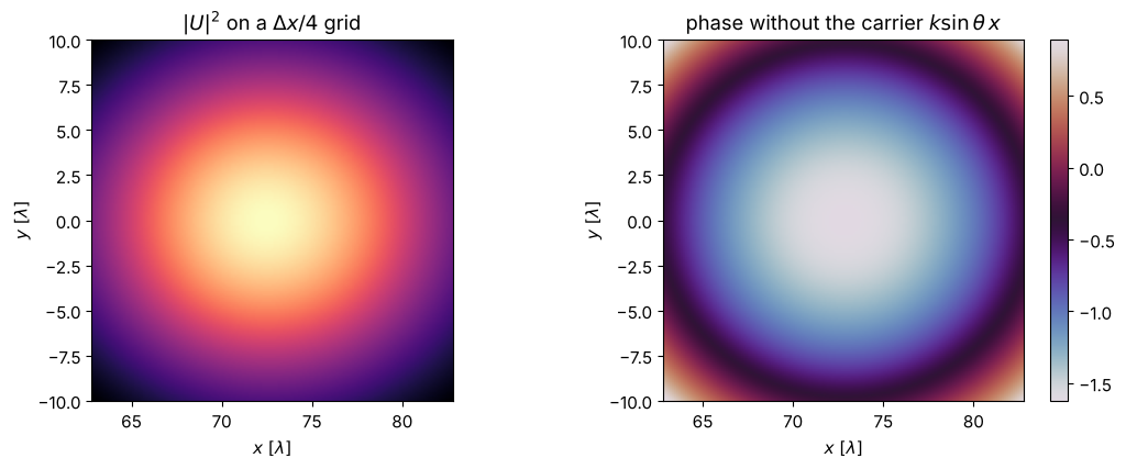
The detector window can also have its own sampling. Below the detector is sampled 4× finer than the source over a \(20\lambda\) wide region around the beam center; the phase shows the tilt and the curvature of the beam (\(w \approx 21\lambda\) at this distance).

x_fine = np.linspace(x0 - 10, x0 + 10, 161)
y_fine = np.linspace(-10, 10, 161)
U_fine, _, _ = shifted_angular_spectrum(source, x, x, z, WL, x_fine, y_fine)
k_carrier = K*np.sin(theta)
X_f, Y_f = np.meshgrid(x_fine, y_fine)

fig, axes = plt.subplots(1, 2, figsize=(11, 4.4))
axes[0].imshow(np.abs(U_fine)**2, extent=[x_fine[0], x_fine[-1], y_fine[0], y_fine[-1]], cmap="magma")
axes[0].set_title(r"$|U|^2$ on a $\Delta x/4$ grid")
im = axes[1].imshow(np.angle(U_fine*np.exp(-1j*k_carrier*X_f)), extent=[x_fine[0], x_fine[-1], y_fine[0], y_fine[-1]], cmap="twilight")
axes[1].set_title(r"phase without the carrier $k\sin\theta\,x$")
plt.colorbar(im, ax=axes[1])
for ax in axes:
    ax.set_xlabel(r"$x\ [\lambda]$"); ax.set_ylabel(r"$y\ [\lambda]$")
plt.tight_layout()

The band limit is what keeps the result free of replicas, but it depends on the spectral spacing \(2\pi/L_\mathrm{pad}\): the band of allowed directions narrows as \((L_\mathrm{in} + L_\mathrm{out})/z\), and once it holds only a few frequency samples, the angular spectrum method is the wrong tool (the function warns). In that regime – the far field of the source – use fresnel_scaled() or far_field().

5. Far field at chosen angles: zooming into a diffraction order

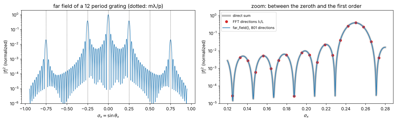
far_field() returns the far field amplitude \(f(\mathbf{s})\) with \(U(r\mathbf{s}) \to f(\mathbf{s})\,e^{ikr}/r\) for \(r \to \infty\),

\[ f(\mathbf{s}) = \frac{k\sigma_z}{2\pi i} \iint U'(x', y')\, e^{-ik(\sigma_x x' + \sigma_y y')}\,dx'\,dy', \]

on an equidistant grid of direction cosines \(\sigma_x = \sin\theta_x\) (no paraxial approximation). The example is a grating of 12 periods \(p = 4\lambda\) illuminated by a plane wave: its orders lie at \(\sin\theta = m\lambda/p\), and between the orders lies the fine structure \(\sin(N\pi u)/\sin(\pi u)\) of a 12-slit interference pattern (10 side lobes of width \(\lambda/(Np)\)). A plain FFT of the \(128\lambda\) window samples the directions with the spacing \(\lambda/L \approx 0.008\), i.e. with about two points per side lobe; far_field() resolves them with any sampling.

p, n_periods, duty = 4.0, 12, 0.5
L, N = 128.0, 1024
x = grid1d(-L/2, L/2, N)
X, Y = np.meshgrid(x, x)
grating = ((np.mod(X, p) < duty*p) & (np.abs(X) < n_periods*p/2) & (np.abs(Y) < 20)).astype(complex)

s_all = np.linspace(-0.95, 0.95, 1901)
f_all, _, _ = far_field(grating, x, x, WL, s_all, np.array([0.0]))
s_order = np.linspace(WL/p - 0.13, WL/p + 0.03, 801)
f_order, _, _ = far_field(grating, x, x, WL, s_order, np.array([0.0]))

# analytic: N-slit interference times the slit envelope; the open
# samples of the discrete grating are summed exactly
dx = x[1] - x[0]
row = grating[N//2]
open_x = x[np.abs(row) > 0]
n_y = np.count_nonzero(np.abs(grating[:, N//2 + 1]) > 0)
def analytic(s):
    s_z = np.sqrt(1 - s**2)
    A = np.exp(-1j*K*np.outer(s, open_x)).sum(axis=1)*dx*n_y*dx
    return K*s_z/(2j*np.pi)*A

fig, axes = plt.subplots(1, 2, figsize=(14, 4.4))
I_max = np.abs(f_all).max()**2
axes[0].semilogy(s_all, np.abs(f_all[0])**2/I_max, "C0", lw=1)
for m in range(-3, 4):
    axes[0].axvline(m*WL/p, color="k", ls=":", lw=0.8)
axes[0].set_ylim(1E-6, 2)
axes[0].set_xlabel(r"$\sigma_x = \sin\theta_x$"); axes[0].set_ylabel(r"$|f|^2$ (normalized)")
axes[0].set_title("far field of a 12 period grating (dotted: mλ/p)")
axes[1].semilogy(s_order, np.abs(analytic(s_order))**2/I_max, color="0.75", lw=5, label="direct sum")
s_fft = frequencies(x)/K
in_zoom = (s_fft >= s_order[0]) & (s_fft <= s_order[-1])
f_fft = far_field(grating, x, x, WL, s_fft[in_zoom], np.array([0.0]))[0][0]
axes[1].semilogy(s_fft[in_zoom], np.abs(f_fft)**2/I_max, "o", color="C3", label="FFT directions λ/L")
axes[1].semilogy(s_order, np.abs(f_order[0])**2/I_max, "C0", label="far_field(), 801 directions")
axes[1].set_xlabel(r"$\sigma_x$"); axes[1].set_ylabel(r"$|f|^2$ (normalized)")
axes[1].set_title("zoom: between the zeroth and the first order")
axes[1].set_ylim(1E-5, 2); axes[1].legend(fontsize=9)
plt.tight_layout()
print("max deviation from the direct sum: {:.1e}".format(np.abs(f_order[0] - analytic(s_order)).max()/np.abs(f_order).max()))

max deviation from the direct sum: 1.7e-11

Summary

• czt() evaluates Fourier sums on any equidistant set of frequencies; zoom_FT() and zoom_inv_FT() wrap it with the pyoptics conventions and agree with FT()/inv_FT() (and with zero padded FFTs) to round-off.

• get_psf(..., x_out, y_out) resolves the PSF on any window without padding: the image grid only sets the pupil sampling.

• fresnel_scaled() and fraunhofer_scaled() free the output grid of the single-transform propagators; they agree with fresnel_rescaling() and fraunhofer() on those grids.

• shifted_angular_spectrum() propagates exactly onto off-axis and rescaled windows; padding to source + detector size together with the band limit removes the replicas.

• far_field() gives the far field in any set of directions, e.g. the fine structure of a single diffraction order.

References

• L. R. Rabiner, R. W. Schafer and C. M. Rader, “The chirp z-transform algorithm”, IEEE Trans. Audio Electroacoust. 17, 86-92 (1969).

• L. I. Bluestein, “A linear filtering approach to the computation of discrete Fourier transform”, IEEE Trans. Audio Electroacoust. 18, 451-455 (1970).

• K. Matsushima, “Shifted angular spectrum method for off-axis numerical propagation”, Opt. Express 18, 18453-18463 (2010).

• J. W. Goodman, Introduction to Fourier Optics, 4th ed., W. H. Freeman (2017).