Telecentricity across the slit: chief ray versus energetic

A lens is telecentric in image space when the light arrives at the wafer centred on the normal, so that defocus blurs the image but does not move it. The usual check follows the chief ray alone. What the wafer sees is the energetic centroid of the cone of light: the chief ray, the real (possibly decentred) pupil, the illumination fill and the transmission of the coated lens together. This notebook compares the two for Caldwell’s KrF lens (NA 0.56) over a 21 × 5 mm slit, and follows the difference into the lithography simulation as pattern shifts through focus.

import time

import numpy as np
import matplotlib.pyplot as plt
from matplotlib.patches import Circle, Rectangle

from pyoptics.coatings import Coating
from pyoptics.materials import Isotropic, extinction_from_absorption
from pyoptics.raytrace import caldwell_krf_lens, fused_silica
from pyoptics.litho import Illumination, LithoSimulation, MaskLayout, Projector, ThinMask, lens

plt.rcParams.update({"figure.dpi": 80, "font.size": 11})
t_start = time.time()

system = caldwell_krf_lens()           # lengths in mm
WL = system.wavelength_nm              # simulation length unit: nm
NA = lens.lens_NA(system)
m = system.paraxial().magnification
n_glass = fused_silica(WL)
R_FIELD = 11.7                         # image field radius (mm)
SLIT_X, SLIT_Y = 10.5, 2.5             # half widths of a 21 x 5 mm slit
print(f"wavelength {WL:.1f} nm, NA {NA:.4f}, magnification {m:.4f}, fused silica n = {n_glass:.4f}")

wavelength 248.3 nm, NA 0.5581, magnification -0.2500, fused silica n = 1.5084

1. Lens, coatings and slit

The lens has 21 fused silica elements, 42 glass–air surfaces. Uncoated, each reflects 4 % at normal incidence and the lens transmits only 17 %; every surface needs an antireflection coating. Four variants, all thin films on every surface (coating= of lens_telecentricity(), from the air side), designed for normal incidence:

coating	layers	R at 0°
uncoated	–	4.1 %
ideal single layer	\(\lambda/4\) of \(n = \sqrt{n_\mathrm{glass}} = 1.228\) (no such material exists)	0
MgF\(_2\) single layer	\(\lambda/4\) of \(n = 1.415\), the lowest index available in the DUV	1.6 %
LaF\(_3\)/MgF\(_2\) V coat	\(\lambda/4\) MgF\(_2\) on \(\lambda/4\) LaF\(_3\) (\(n = 1.69\))	0.1 %

Fused silica for KrF absorbs a little; we take an internal transmission of 99.8 % per cm (\(\alpha = 0.002\)/cm), as an absorbing medium (materials.Isotropic(n, k)) behind every glass surface. The coated lens of the later sections is the V coat with this absorption.

wl = system.wavelength                 # mm
N_MGF2, N_LAF3 = 1.415, 1.69
coatings = {"uncoated": None,
            "ideal single layer": lens.quarter_wave_coating(n_glass, wl),
            "MgF$_2$ single layer": [(N_MGF2, wl/(4*N_MGF2))],
            "LaF$_3$/MgF$_2$ V coat": [(N_MGF2, wl/(4*N_MGF2)), (N_LAF3, wl/(4*N_LAF3))]}
V_COAT = coatings["LaF$_3$/MgF$_2$ V coat"]

ALPHA = 0.002/10                        # 1/mm
k_glass = extinction_from_absorption(ALPHA, wl)
glass = [i for i in range(len(system.surfaces)) if system.n[i + 1] > 1.2]
absorbing = {i: Isotropic(n_glass, k_glass) for i in glass}
path = sum(s.thickness for i, s in enumerate(system.surfaces) if i in glass)
print(f"{len(glass)} elements, {path:.0f} mm of glass on axis: internal transmission "
      f"{np.exp(-ALPHA*path):.3f}")


def max_angles_in_air(system, fields, N=21):
    """Largest angle of incidence (in air) on each surface over the pupil and the fields."""
    n = system.n
    frames = system.frames()[0]
    p = np.linspace(-1, 1, N)
    PX, PY = np.meshgrid(p, p)
    inside = PX**2 + PY**2 <= 1
    worst = np.zeros(len(system.surfaces))
    for f in fields:
        b = system.trace_pupil((0.0, f/m), PX[inside], PY[inside])
        for i, s in enumerate(system.surfaces):
            o, R = frames[i]
            Q = (b.points[i + 1][b.valid] - o) @ R
            cos_i = np.abs(np.sum(s.normal(Q)*(b.directions[i][b.valid] @ R), axis=-1))
            worst[i] = max(worst[i], np.max(max(n[i], n[i + 1])*np.sqrt(1 - cos_i**2)))
    return np.degrees(np.arcsin(np.clip(worst, 0, 1)))


aoi = max_angles_in_air(system, (0.0, R_FIELD))
fig, axes = plt.subplots(1, 3, figsize=(18, 4.3), gridspec_kw={"width_ratios": [1.6, 1, 1]})
system.draw(ax=axes[0], fields=[(0.0, 0.0), (0.0, R_FIELD/m)], n_rays=5)
axes[0].set_title("Caldwell's KrF lens, NA 0.56, 4x (object left)")
ax = axes[1]
ax.add_patch(Circle((0, 0), R_FIELD, fill=False, lw=2, label="image field Ø 23.4 mm"))
ax.add_patch(Rectangle((-SLIT_X, -SLIT_Y), 2*SLIT_X, 2*SLIT_Y, alpha=0.3, color="C1",
                       label="slit 21 × 5 mm"))
ax.annotate("", xy=(0, 8.5), xytext=(0, 4), arrowprops=dict(arrowstyle="->", lw=2))
ax.text(0.4, 6, "scan", fontsize=10)
ax.set_aspect("equal"); ax.set_xlim(-13, 13); ax.set_ylim(-13, 13)
ax.set_xlabel("x [mm]"); ax.set_ylabel("y [mm]"); ax.legend(fontsize=8, loc="lower left")
ax.set_title("image field and slit (wafer side)")
ax = axes[2]
angles = np.radians(np.linspace(0, 85, 171))
for k, (name, layers) in enumerate(coatings.items()):
    out = Coating(layers or []).power(angles, 1.0, n_glass, wl)
    ax.plot(np.degrees(angles), 100*(out["R_s"] + out["R_p"])/2, color=f"C{k}", label=name)
    ax.plot(np.degrees(angles), 100*out["R_p"], ":", color=f"C{k}", lw=1)
for a in aoi:
    ax.axvline(a, color="0.6", lw=0.6, zorder=0)
ax.set_xlabel("angle of incidence in air [°]"); ax.set_ylabel("reflectance [%]")
ax.set_ylim(0, 12); ax.legend(fontsize=8)
ax.set_title("one surface: unpolarized (solid), p (dotted);\ngrey: largest angle on each lens surface")
fig.tight_layout()
print("largest angles of incidence on the surfaces (deg):", np.round(np.sort(aoi)[::-1][:8], 1))

21 elements, 565 mm of glass on axis: internal transmission 0.893

largest angles of incidence on the surfaces (deg): [82.9 65.5 51.7 51.5 50.5 50.  47.5 45.8]

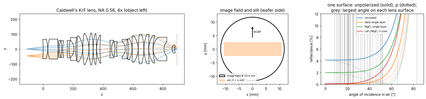
The single layer coatings and the V coat work at normal incidence, but many surfaces see angles of 30–50° and a few, steep surfaces at the rim of the field even 65–83° (grey lines), where the reflectance rises quickly and differs for s and p. Off axis, the rays above and below the chief ray meet these surfaces at different angles: this is where the asymmetric apodization comes from.

The slit: 21 × 5 mm fits into the 23.4 mm image field of this stepper lens (a scanner lens of 4x has a 26 × 8 mm slit, but the principle is the same). Mask and wafer move along \(y\); every wafer point sees all \(y\) of the slit at its slit position \(x\).

2. Chief ray telecentricity

Caldwell’s paper calls the lens telecentric on both sides; the chief rays of the model (stop on surface 30, see caldwell_krf_lens()) leave it within a few mrad of the axis. The lens is rotationally symmetric, so the chief ray tilt is radial and a function of the field radius \(r\) only.

def chief_slope(field):
    """Image space chief ray slope (dx/dz, dy/dz) at an image field point."""
    b = system.trace_pupil(np.asarray(field, dtype=float)/m, 0.0, 0.0)
    d = system._image_hits(b)[1][0]
    return d[:2]/d[2]


r = np.linspace(0, R_FIELD, 40)
chief_r = np.array([chief_slope((x, 0.0))[0] for x in r])*1e3
xs = np.linspace(-SLIT_X, SLIT_X, 15)
ys = np.linspace(-SLIT_Y, SLIT_Y, 5)
F = np.array([(x, y) for y in ys for x in xs])
C = np.array([chief_slope(f) for f in F])*1e3

fig, axes = plt.subplots(1, 2, figsize=(16, 4.2), gridspec_kw={"width_ratios": [1, 1.6]})
axes[0].plot(r, chief_r, "C0-")
axes[0].axvspan(SLIT_X, np.hypot(SLIT_X, SLIT_Y), color="C1", alpha=0.2, label="slit corners")
axes[0].axhline(0, color="k", lw=0.5)
axes[0].set_xlabel("field radius r [mm]"); axes[0].set_ylabel("radial chief ray slope [mrad]")
axes[0].set_title("chief ray telecentricity"); axes[0].legend(fontsize=9)
q = axes[1].quiver(F[:, 0], F[:, 1], C[:, 0], C[:, 1], angles="xy", scale_units="xy", scale=1,
                   width=0.003)
axes[1].quiverkey(q, 0.85, 1.05, 2, "2 mrad", labelpos="E")
axes[1].add_patch(Rectangle((-SLIT_X, -SLIT_Y), 2*SLIT_X, 2*SLIT_Y, fill=False, color="C1"))
axes[1].set_aspect("equal"); axes[1].set_xlim(-12, 12); axes[1].set_ylim(-4, 4)
axes[1].set_xlabel("x [mm]"); axes[1].set_ylabel("y [mm]")
axes[1].set_title(f"chief ray slopes across the slit, max {np.max(np.hypot(*C.T)):.1f} mrad")
fig.tight_layout()

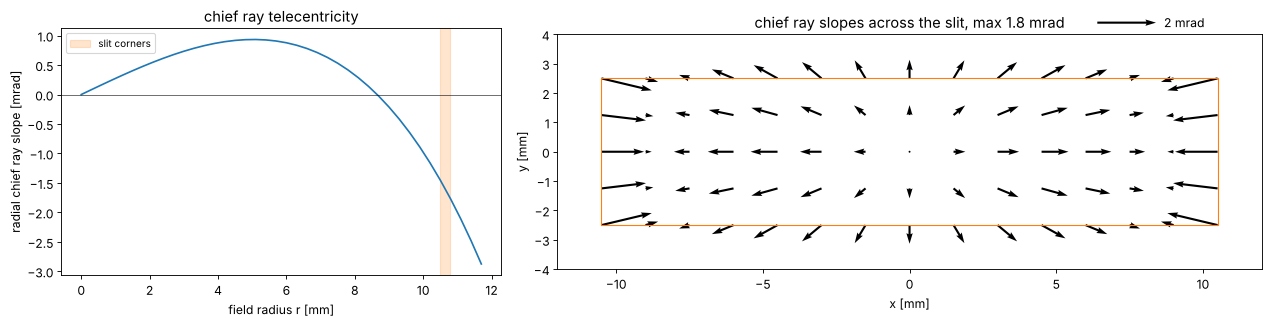
The chief ray tilt stays below about 2 mrad in the slit; it changes sign at about 9 mm (the design balances it over the field). By the chief ray alone this is a good telecentric lens: 100 nm of defocus move the image by at most 0.2 nm.

3. The cone of light

The chief ray is the centre of the stop; the light is the whole cone that passes the stop and, before that, what the illuminator puts into it. lens_telecentricity() traces a grid of rays through the stop from the object point and weights each ray with its etendue, the object side solid angle of its tube \(\mathrm{d}u_x\,\mathrm{d}u_y\) of direction sines (from the Jacobian of the ray aiming), and with the illumination fill: a uniform source of radius \(\sigma\) (in units of the object side NA, centred on the object side chief ray), or fill=None for the whole cone that the stop passes (the light diffracted by a small feature, or incoherent light). Its geometric result is the centroid of the image side slopes without losses, energetic the same with the transmission of each ray.

First the pupil itself at the slit edge, \(x = 10.5\) mm: the image side directions of the rays relative to the chief ray, in units of the NA, and the etendue weight of each ray.

X_EDGE = SLIT_X
full_edge = lens.lens_telecentricity(system, (X_EDGE, 0.0), N=64)
axis = lens.lens_telecentricity(system, (0.0, 0.0), N=64)
phi = np.linspace(0, 2*np.pi, 361)

fig, axes = plt.subplots(1, 3, figsize=(17, 4.8))
for ax, t, title in ((axes[0], axis, "on axis"), (axes[1], full_edge, f"x = {X_EDGE} mm")):
    im = ax.tripcolor(t.P_x, t.P_y, t.weight*len(t.weight), shading="gouraud", cmap="viridis",
                      vmin=0.8, vmax=1.25)
    ax.plot(np.cos(phi), np.sin(phi), "w--", lw=1, label="circle about the chief ray")
    ax.plot(0, 0, "w+", ms=12)
    ax.set_aspect("equal"); ax.set_xlim(-1.08, 1.08); ax.set_ylim(-1.08, 1.08)
    ax.set_xlabel("$P_x$ (relative to the chief ray)"); ax.set_ylabel("$P_y$")
    ax.set_title(f"{title}: etendue weight of the rays")
plt.colorbar(im, ax=axes[1], label="weight × number of rays")
axes[0].legend(fontsize=8, loc="lower left")
x_rim = [full_edge.P_x.min(), full_edge.P_x.max()]
print(f"x = {X_EDGE} mm: the cone reaches from P_x = {x_rim[0]:.3f} to {x_rim[1]:.3f}, "
      f"centre {np.mean(x_rim):+.3f} (in NA units)")

# the centroid against the illumination fill
sigmas = np.linspace(0.1, 1.0, 10)
cases = [(s, lens.lens_telecentricity(system, (X_EDGE, 0.0), N=64, fill=s)) for s in sigmas]
ax = axes[2]
ax.plot(sigmas, [1e3*t.geometric[0] for _, t in cases], "o-", label="centroid of the cone, fill σ")
ax.axhline(1e3*full_edge.geometric[0], color="C3", ls="--", label="whole cone of the stop")
ax.axhline(1e3*full_edge.chief[0], color="k", lw=1, label="chief ray")
ax.set_xlabel("illumination σ"); ax.set_ylabel("slope $x$ [mrad]")
ax.set_title(f"geometric telecentricity at x = {X_EDGE} mm (no losses)"); ax.legend(fontsize=9)
fig.tight_layout()
for s, t in cases[1::3]:
    print(f"sigma {s:.1f}: centroid {1e3*t.geometric[0]:+.2f} mrad")
print(f"whole cone: {1e3*full_edge.geometric[0]:+.2f} mrad, chief ray {1e3*full_edge.chief[0]:+.2f} mrad")

x = 10.5 mm: the cone reaches from P_x = -1.013 to 0.902, centre -0.056 (in NA units)

sigma 0.2: centroid -1.48 mrad
sigma 0.5: centroid -1.67 mrad
sigma 0.8: centroid -1.49 mrad
whole cone: -36.13 mrad, chief ray -1.45 mrad

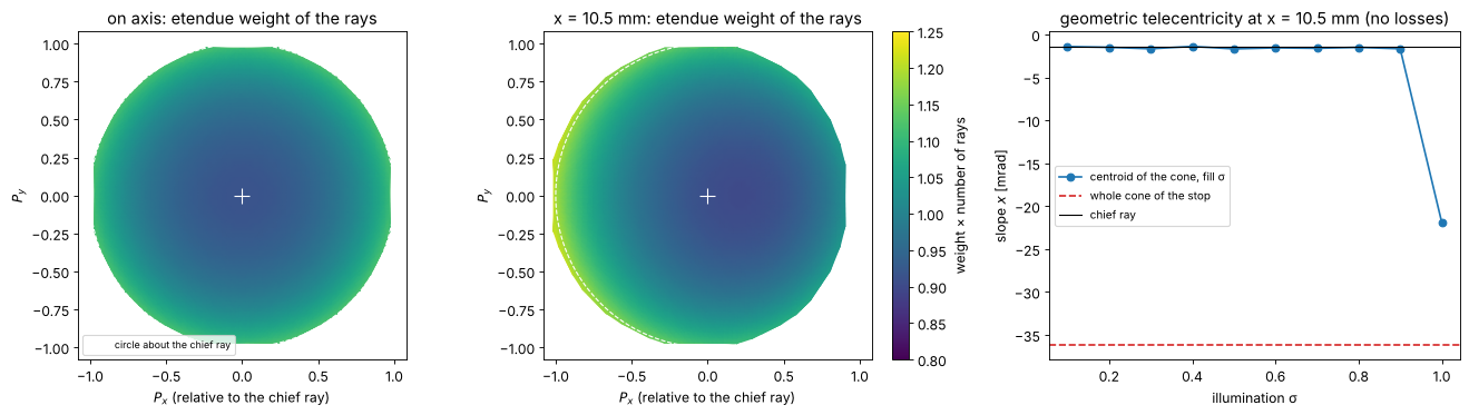
Two findings:

• The pupil is decentred. On axis the cone is a disk about the chief ray. At the slit edge it is shifted by about 5 % of its radius to \(-x\) (its rim reaches \(P_x \approx -1.01\) on one side and \(+0.90\) on the other): the chief ray goes through the centre of the stop, but seen from the off-axis object point the stop is not centred on it (pupil coma of the front group). The whole cone of the stop is therefore tilted by about −36 mrad, 25 times the chief ray. This depends on where the stop is, which Caldwell’s paper does not say: with a stop on the almost flat surface 31 instead of the strongly curved surface 30 (whose rim lies 18 mm in front of its vertex) the chief rays are as telecentric, and the decentration is about 2.5 times smaller (at a somewhat smaller NA).

• A symmetric illumination is not affected. A source of \(\sigma \le 0.9\) centred on the object side chief ray stays inside the stop, and its cone is centred on the chief ray in image space too, to a few tenths of a mrad: the lens maps object side directions to image side directions linearly (with the factor 1/m, the sine condition), so a disk stays a disk about the chief ray. At σ = 1 the disk touches the decentred stop on one side and the centroid jumps.

So the light of the illuminator (the zero order of a mask) arrives telecentric, while light diffracted to the rim of the pupil (small features) sees the decentred stop. Without losses, this is all of the geometry; now the transmission.

4. Apodization and energetic telecentricity

The polarization ray trace gives the power transmission of every ray for unpolarized light: Fresnel coefficients or the thin film stack on every surface, and the absorption on the path through the glass. Relative to the chief ray, at the slit edge:

variants = dict(coatings)
variants["V coat + absorption"] = V_COAT


def trace(field, name, N=48, fill=None):
    c = variants[name]
    media = absorbing if name == "V coat + absorption" else None
    return lens.lens_telecentricity(system, field, N=N, fill=fill, coating=c, birefringent=media)


edge = {name: trace((X_EDGE, 0.0), name) for name in variants}
fig, axes = plt.subplots(1, 5, figsize=(20, 4.0))
for ax, (name, t) in zip(axes, edge.items()):
    rel = t.T/np.max(t.T)
    im = ax.tripcolor(t.P_x, t.P_y, rel, shading="gouraud", cmap="magma")
    ax.set_aspect("equal"); ax.set_xticks([]); ax.set_yticks([])
    ax.set_title(f"{name}\nmean T = {t.transmission:.3f}", fontsize=10)
    plt.colorbar(im, ax=ax, shrink=0.8)
fig.suptitle(f"power transmission over the pupil at x = {X_EDGE} mm (relative to its maximum)", y=1.02)
fig.tight_layout()

• Uncoated, the transmission rises towards the rim in \(x\), most on the \(+x\) side, where the rays meet the surfaces closer to Brewster’s angle (\(p\) is transmitted better; the radial diattenuation of notebook 38), and falls towards \(\pm y\).

• The coatings have the opposite trend: designed for normal incidence, they reflect more at large angles, so the transmission falls towards the rim of the pupil, by 1–2 % for the single layers and 4 % for the V coat, whose reflectance rises fastest with the angle (section 1), and more on the \(+x\) side.

• The absorption takes 11 % on axis and varies with the glass path across the pupil; it partly fills in the rim on the \(-x\) side.

Off axis, none of these patterns is symmetric about the chief ray. Its tilt part moves the energy centroid. The energetic telecentricity, the centroid weighted with this transmission, against the geometric centroid, for the whole cone and for a conventional illumination of \(\sigma = 0.8\):

xs_half = np.linspace(0, SLIT_X, 8)
SIGMA = 0.8
rows = {}
for name in variants:
    for fill in (None, SIGMA):
        rows[name, fill] = [trace((x, 0.0), name, N=48, fill=fill) for x in xs_half]

fig, axes = plt.subplots(1, 2, figsize=(16, 4.5), sharey=True)
for ax, fill, title in ((axes[0], SIGMA, f"illumination σ = {SIGMA}"),
                        (axes[1], None, "whole cone of the stop")):
    for k, name in enumerate(variants):
        d = [1e3*(t.energetic[0] - t.geometric[0]) for t in rows[name, fill]]
        ax.plot(xs_half, d, "o-", color=f"C{k}", ms=4, label=name)
    ax.axhline(0, color="k", lw=0.5)
    ax.set_xlabel("slit position x [mm]"); ax.set_title(title)
axes[0].set_ylabel("energetic − geometric centroid [mrad]")
axes[0].legend(fontsize=9)
fig.tight_layout()
for name in variants:
    t = rows[name, SIGMA][-1]
    print(f"{name:26s} x = {SLIT_X} mm, sigma {SIGMA}: chief {1e3*t.chief[0]:+.2f}, geometric "
          f"{1e3*t.geometric[0]:+.2f}, energetic {1e3*t.energetic[0]:+.2f} mrad")

uncoated                   x = 10.5 mm, sigma 0.8: chief -1.45, geometric -1.49, energetic -1.04 mrad
ideal single layer         x = 10.5 mm, sigma 0.8: chief -1.45, geometric -1.49, energetic -1.92 mrad
MgF$_2$ single layer       x = 10.5 mm, sigma 0.8: chief -1.45, geometric -1.49, energetic -1.74 mrad
LaF$_3$/MgF$_2$ V coat     x = 10.5 mm, sigma 0.8: chief -1.45, geometric -1.49, energetic -2.51 mrad
V coat + absorption        x = 10.5 mm, sigma 0.8: chief -1.45, geometric -1.49, energetic -2.27 mrad

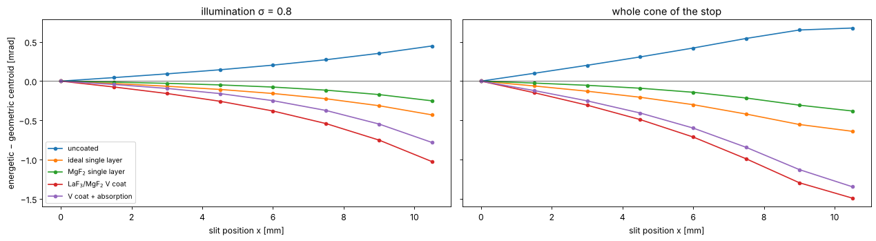
The apodization moves the centroid by up to 1 mrad for the illumination and 1.5 mrad for the whole cone at the slit edge, the same order as the chief ray telecentricity itself (−1.5 mrad there), and with a sign that depends on the coating: the bare lens tilts the light outwards (+x, towards the transmission rise near Brewster’s angle), every coating tilts it inwards, the V coat most, the MgF\(_2\) single layer least. The absorption works against the V coat a little. The whole cone feels more, since the rim of the pupil carries the strongest apodization.

A lens that is telecentric by its chief ray can thus be off by a few mrad energetically, and the coating design is part of the telecentricity budget. From here on the lens is the coated lens (V coat with absorption).

5. Across the slit, static and scanned

Over the whole slit, for three fills: conventional σ = 0.8, annular 0.8/0.5 and the whole cone. The lens is rotationally symmetric, so the slopes are radial: the \(x\) component is odd in \(x\), the \(y\) component odd in \(y\).

def annular(u_x, u_y, outer=0.8, inner=0.5, h=2/47):
    """Annular fill, edges smoothed over one step of the 48 x 48 pupil grid (as for a number sigma)."""
    rho = np.hypot(u_x, u_y)
    return np.clip((outer - rho)/h + 0.5, 0, 1)*np.clip((rho - inner)/h + 0.5, 0, 1)


fills = {"conventional σ 0.8": 0.8, "annular 0.8/0.5": annular, "whole cone": None}
ys_half = np.linspace(0, SLIT_Y, 3)
slit = {name: [[trace((x, y), "V coat + absorption", N=48, fill=f) for x in xs_half] for y in ys_half]
        for name, f in fills.items()}


def component(results, key, i):
    return np.array([[1e3*getattr(t, key)[i] for t in row] for row in results])


fig, axes = plt.subplots(1, 3, figsize=(18, 4.5))
chief_x = component(slit["whole cone"], "chief", 0)[0]
for k, (name, res) in enumerate(slit.items()):
    ax = axes[1] if name == "whole cone" else axes[0]
    ax.plot(xs_half, component(res, "energetic", 0)[0], "o-", color=f"C{k}", ms=4, label=f"energetic, {name}")
    ey = component(res, "energetic", 1)
    axes[2].plot(xs_half, ey[-1], "o-", color=f"C{k}", ms=4, label=f"energetic, {name}")
for ax in axes[:2]:
    ax.plot(xs_half, chief_x, "k--", label="chief ray")
axes[2].plot(xs_half, component(slit["whole cone"], "chief", 1)[-1], "k--", label="chief ray")
axes[0].set_title("x slope at y = 0: the illumination")
axes[1].set_title("x slope at y = 0: the whole cone")
axes[2].set_title(f"y slope at the slit border y = {SLIT_Y} mm")
for ax in axes:
    ax.set_xlabel("slit position x [mm]"); ax.set_ylabel("slope [mrad]"); ax.axhline(0, color="k", lw=0.5)
    ax.legend(fontsize=8)
fig.tight_layout()
for name, res in list(slit.items())[:2]:
    ex = component(res, "energetic", 0)
    scanned = np.average(ex, axis=0, weights=[1, 2, 1])   # y = 0, +-1.25, +-2.5 mm (trapezoid rule)
    print(f"{name}: scanned minus static x slope, largest {np.max(np.abs(scanned - ex[0])):.2f} mrad")
for name, res in slit.items():
    ex, cx = component(res, "energetic", 0), component(res, "chief", 0)
    print(f"{name:20s}: energetic x slope at the slit edge {ex[0, -1]:+.2f} mrad "
          f"(chief ray {cx[0, -1]:+.2f}), largest |energetic - chief| in the slit "
          f"{np.max(np.abs(ex - cx)):.2f} mrad")

conventional σ 0.8: scanned minus static x slope, largest 0.14 mrad
annular 0.8/0.5: scanned minus static x slope, largest 0.17 mrad
conventional σ 0.8  : energetic x slope at the slit edge -2.27 mrad (chief ray -1.45), largest |energetic - chief| in the slit 0.94 mrad
annular 0.8/0.5     : energetic x slope at the slit edge -2.48 mrad (chief ray -1.45), largest |energetic - chief| in the slit 1.23 mrad
whole cone          : energetic x slope at the slit edge -38.01 mrad (chief ray -1.45), largest |energetic - chief| in the slit 37.44 mrad

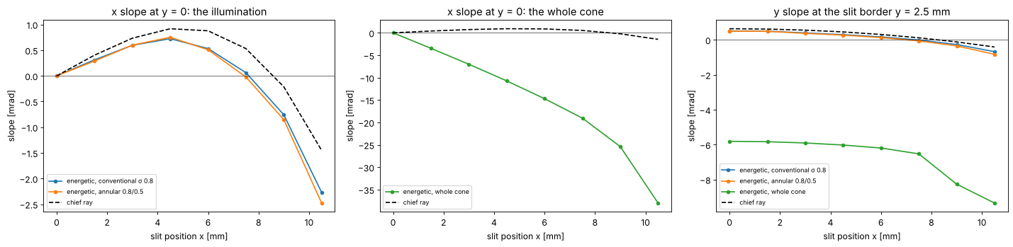
• For the illumination the energetic telecentricity follows the chief ray, with an offset of up to about 1 mrad (conventional) to 2 mrad (annular, whose light sits at the larger angles where the coatings apodize most) from the apodization, largest at the slit edge.

• The whole cone is dominated by the decentred stop: up to −38 mrad.

• Scanning averages over \(y\). The \(x\) slope barely changes with \(y\) (the slit is short in \(y\)), so the scanned value is close to the static one at \(y = 0\) (printed above). The \(y\) slope is odd in \(y\): it averages to zero, but at the slit border it is about ±0.6 mrad for the illumination and up to ±9 mrad for the whole cone. A wafer point that is out of focus by \(z\) receives images moved by \(z\,\theta_y(y)\) during the scan: the image of horizontal lines is blurred by \(z\,\Delta\theta_y\) instead of moved (image fading), about 0.1 nm at \(z\) = 100 nm for the illumination, up to 2 nm for light at the rim of the pupil.

6. Impact: pattern shift through focus

The lithography simulation describes the lens by its pupil on coordinates about the chief ray. lens_apodization() gives that pupil from the ray trace: zero outside the real (decentred) pupil and the square root of the relative transmission inside, for Projector(apodization=...). The projector gets an NA 6 % larger than the lens so that its disk contains the shifted pupil; the illumination σ is scaled accordingly. The chief ray tilt is not in the pupil (its coordinates are relative to the chief ray) and is added as \(z\tan\theta_\mathrm{chief}\), as in through_slit() of notebook 33.

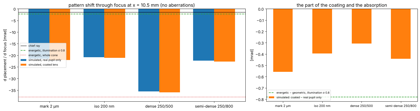
Four patterns, binary mask, conventional illumination σ = 0.8, at the slit edge, first without the lens aberrations (the pupil and the apodization only), placement of the feature centre through ±300 nm of focus:

• a large 2 µm line (an alignment or overlay mark),

• an isolated 200 nm line,

• dense 250 nm lines at a pitch of 500 nm and semi-dense ones at 800 nm.

Each pattern twice: with the real pupil only (decentred, transmission 1) and with the coated lens (decentred pupil and the transmission).

K = 1.06
NA_P = K*NA
FOCI = np.linspace(-300, 300, 7)
patterns = {"mark 2 µm": MaskLayout.iso_line(2000.0, 8000.0),
            "iso 200 nm": MaskLayout.iso_line(200.0, 3000.0),
            "dense 250/500": MaskLayout.lines_spaces(500.0, 250.0),
            "semi-dense 250/800": MaskLayout.lines_spaces(800.0, 250.0)}
ill = Illumination.conventional(SIGMA/K, n_samples=21)


def apodized_projector(field, transmission=True, aberrations=False):
    apo = lens.lens_apodization(system, field, N=48, NA=NA_P, coating=V_COAT, birefringent=absorbing,
                                transmission=transmission)
    z = lens.lens_aberrations(system, field, NA=NA_P, N=40).zernikes if aberrations else None
    return Projector(NA_P, WL, magnification=4.0, apodization=apo, zernikes=z)


def placement_through_focus(layout, projector, field, illumination=ill):
    sim = LithoSimulation(layout, ThinMask.binary(), illumination, projector)
    r = lens.feature_response(sim, threshold=0.3, foci=FOCI)
    return r.placement_focus + FOCI*chief_slope(field)[0]   # plus the chief ray tilt


def slope_of(placement):
    return 1e3*np.polyfit(FOCI, placement, 1)[0]            # mrad


field = (X_EDGE, 0.0)
projectors = {"real pupil only": apodized_projector(field, transmission=False),
              "coated lens": apodized_projector(field)}
slopes = {(name, mode): slope_of(placement_through_focus(layout, P, field))
          for name, layout in patterns.items() for mode, P in projectors.items()}
on_axis = apodized_projector((0.0, 0.0))
print("on axis:", {name: round(slope_of(placement_through_focus(layout, on_axis, (0.0, 0.0))), 4)
                   for name, layout in patterns.items()})
t_ill = slit["conventional σ 0.8"][0][-1]
t_full = slit["whole cone"][0][-1]
coating_part = 1e3*(t_ill.energetic[0] - t_ill.geometric[0])

fig, axes = plt.subplots(1, 2, figsize=(17, 4.6), gridspec_kw={"width_ratios": [1.5, 1]})
idx = np.arange(len(patterns))
ax = axes[0]
for k, mode in enumerate(projectors):
    ax.bar(idx + (k - 0.5)*0.38, [slopes[n, mode] for n in patterns], 0.38, label=f"simulated, {mode}")
ax.axhline(1e3*t_ill.chief[0], color="k", lw=1, label="chief ray")
ax.axhline(1e3*t_ill.energetic[0], color="C2", ls="--", label=f"energetic, illumination σ {SIGMA}")
ax.axhline(1e3*t_full.energetic[0], color="C3", ls=":", label="energetic, whole cone")
ax.set_xticks(idx); ax.set_xticklabels(patterns); ax.axhline(0, color="k", lw=0.5)
ax.set_ylabel("d placement / d focus [mrad]"); ax.legend(fontsize=8, loc="center left")
ax.set_title(f"pattern shift through focus at x = {X_EDGE} mm (no aberrations)")
ax = axes[1]
ax.bar(idx, [slopes[n, "coated lens"] - slopes[n, "real pupil only"] for n in patterns], 0.5,
       color="C1", label="simulated: coated − real pupil only")
ax.axhline(coating_part, color="C2", ls="--",
           label=f"energetic − geometric, illumination σ {SIGMA}")
ax.set_xticks(idx); ax.set_xticklabels(patterns, fontsize=9); ax.axhline(0, color="k", lw=0.5)
ax.set_ylabel("[mrad]"); ax.set_title("the part of the coating and the absorption")
ax.legend(fontsize=8)
fig.tight_layout()
for name in patterns:
    print(f"{name:20s}: real pupil only {slopes[name, 'real pupil only']:+7.2f}, coated "
          f"{slopes[name, 'coated lens']:+7.2f} mrad")
print(f"chief ray {1e3*t_ill.chief[0]:+.2f}, energetic: illumination {1e3*t_ill.energetic[0]:+.2f}, "
      f"whole cone {1e3*t_full.energetic[0]:+.2f}; coating part (illumination) {coating_part:+.2f} mrad")

on axis: {'mark 2 µm': np.float64(0.0), 'iso 200 nm': np.float64(0.0), 'dense 250/500': np.float64(0.0), 'semi-dense 250/800': np.float64(0.0)}
mark 2 µm           : real pupil only  -21.47, coated  -22.03 mrad
iso 200 nm          : real pupil only  -20.78, coated  -21.18 mrad
dense 250/500       : real pupil only  -35.61, coated  -35.92 mrad
semi-dense 250/800  : real pupil only  -22.27, coated  -22.71 mrad
chief ray -1.45, energetic: illumination -2.27, whole cone -38.01; coating part (illumination) -0.78 mrad

• On axis nothing moves: the pupil is symmetric.

• At the slit edge every pattern moves through focus by −21 to −36 mrad, 15–25 times the chief ray and ten times the energetic telecentricity of the illumination. Even the large mark, whose light is mostly the centred illumination, moves this much: its edges diffract light out to the rim of the pupil, and there the decentred pupil clips it on one side. The dense lines (first orders at \(\lambda/(p\,\mathrm{NA}) = 0.89\), spread by σ = 0.8 to the rim) move most.

• The coating adds −0.3 to −0.6 mrad, the same sign and about half to three quarters of the energetic estimate of the illumination (−0.8 mrad). A smooth apodization acts mostly as a reweighting of the source points, i.e. as an energetic tilt of the illumination; the diffracted light sees the tilt too, but differently for each pattern.

So the energetic telecentricity of the illumination is the right measure for smooth transmission errors (coatings, absorption), while the geometry of the pupil rim has to enter the imaging itself: neither the chief ray nor a centroid predicts it. (A centroid of the diffracted light is not a good predictor either: edges are made of the high spatial frequencies, and how much each frequency moves an edge depends on the pattern and the threshold.)

With the lens aberrations, across the slit

The full lens model: the Fringe Zernikes of the ray trace at each slit position (lens_aberrations() on the same pupil coordinates), the decentred pupil with its transmission, and the chief ray tilt. Through focus at the slit centre and edge, and the slope of a linear fit across the slit (static image, \(y = 0\); section 5 showed that scanning changes little here):

xs_slit = np.linspace(0, SLIT_X, 6)
curves, slit_slopes = {}, {name: [] for name in patterns}
for x in xs_slit:
    P = apodized_projector((x, 0.0), aberrations=True)
    for name, layout in patterns.items():
        pl = placement_through_focus(layout, P, (x, 0.0))
        curves[name, x] = pl
        slit_slopes[name].append(slope_of(pl))

fig, axes = plt.subplots(1, 3, figsize=(18, 4.5))
for k, name in enumerate(patterns):
    for ax, x in zip(axes[:2], xs_slit[-2:]):
        pl = curves[name, x]
        ax.plot(FOCI, pl - pl[len(FOCI)//2], "o-", color=f"C{k}", ms=4, label=name)
    axes[2].plot(xs_slit, slit_slopes[name], "o-", color=f"C{k}", ms=4, label=name)
axes[2].plot(xs_slit, [1e3*chief_slope((x, 0.0))[0] for x in xs_slit], "k--", label="chief ray")
for ax, x in zip(axes[:2], xs_slit[-2:]):
    ax.set_xlabel("focus [nm]"); ax.set_ylabel("placement − placement at focus 0 [nm]")
    ax.set_title(f"x = {x} mm, full lens model"); ax.axhline(0, color="k", lw=0.5)
axes[0].legend(fontsize=8)
axes[2].set_xlabel("slit position x [mm]"); axes[2].set_ylabel("d placement / d focus [mrad]")
axes[2].set_title("slope of the linear fit over ±300 nm"); axes[2].axhline(0, color="k", lw=0.5)
axes[2].legend(fontsize=8)
fig.tight_layout()
for name in patterns:
    print(f"{name:20s}: slope across the slit [mrad]", np.round(slit_slopes[name], 1))
mark, dense = curves["mark 2 µm", SLIT_X], curves["dense 250/500", SLIT_X]
d = (mark - mark[3]) - (dense - dense[3])
print(f"mark to dense lines offset at x = {SLIT_X} mm, focus -100 / +100 nm: {np.interp(-100, FOCI, d):+.1f} / "
      f"{np.interp(100, FOCI, d):+.1f} nm")

mark 2 µm           : slope across the slit [mrad] [  0.   -2.1  -2.8  -5.9 -19.2 -31.2]
iso 200 nm          : slope across the slit [mrad] [  0.   -3.3  -2.   -4.8 -22.9 -32.3]
dense 250/500       : slope across the slit [mrad] [  0.   -6.1  -6.5 -10.1 -27.2 -45.6]
semi-dense 250/800  : slope across the slit [mrad] [  0.   -3.6  -1.9  -6.4 -25.1 -37.9]
mark to dense lines offset at x = 10.5 mm, focus -100 / +100 nm: -1.5 / +1.3 nm

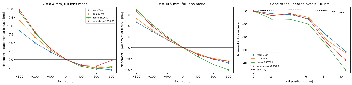
• With the aberrations the slopes at the slit edge grow to −31 to −46 mrad: the lens has about 0.1 waves of coma and astigmatism there, and coma together with defocus moves the image through focus as well (the curves are not straight).

• Across the slit the shifts stay within ±10 mrad up to about 6 mm and then grow steeply with the decentration of the pupil; the chief ray stays within 1.5 mrad everywhere.

• The patterns move differently. At the slit edge, 100 nm of defocus moves the mark and the dense lines apart by about 1.4 nm: an overlay error between the alignment and overlay marks and the device patterns that no measurement on the marks reveals.

7. Compensation by the illuminator

Scanners can tilt the illumination per slit position (the illuminator’s pupil fill is moved slightly off centre, e.g. by its field-dependent optics). A source moved by \(\delta\sigma\) tilts the zero order cone by about \(\delta\sigma\,\mathrm{NA}\). We choose \(\delta\sigma\) at the slit edge so that the mark does not move through focus (full lens model) and look at what happens to the other patterns:

P_edge = apodized_projector(field, aberrations=True)


def shifted(delta):
    return Illumination(ill.s_x + delta, ill.s_y, ill.weights)


def mark_slope(delta):
    return slope_of(placement_through_focus(patterns["mark 2 µm"], P_edge, field, shifted(delta)))


s0, s1 = mark_slope(0.0), mark_slope(0.01)
delta = -0.01*s0/(s1 - s0)
print(f"mark slope {s0:+.2f} mrad, {(s1 - s0)/0.01:.0f} mrad per unit sigma "
      f"(NA of the projector: {1e3*NA_P:.0f} mrad); delta sigma = {delta:+.4f} (in units of the projector NA)")
after = {name: slope_of(placement_through_focus(layout, P_edge, field, shifted(delta)))
         for name, layout in patterns.items()}
before = {name: slit_slopes[name][-1] for name in patterns}

fig, ax = plt.subplots(figsize=(10, 4.2))
ax.bar(idx - 0.2, [before[n] for n in patterns], 0.4, label="centred illumination")
ax.bar(idx + 0.2, [after[n] for n in patterns], 0.4, label=f"illumination moved by δσ = {delta:+.3f}")
ax.set_xticks(idx); ax.set_xticklabels(patterns); ax.axhline(0, color="k", lw=0.5)
ax.set_ylabel("d placement / d focus [mrad]"); ax.legend(fontsize=9)
ax.set_title(f"x = {X_EDGE} mm, full lens model")
fig.tight_layout()
for name in patterns:
    print(f"{name:20s}: {before[name]:+7.2f} -> {after[name]:+7.2f} mrad")

mark slope -31.24 mrad, 372 mrad per unit sigma (NA of the projector: 592 mrad); delta sigma = +0.0840 (in units of the projector NA)

mark 2 µm           :  -31.24 ->   -0.06 mrad
iso 200 nm          :  -32.27 ->   -7.02 mrad
dense 250/500       :  -45.65 ->  -27.01 mrad
semi-dense 250/800  :  -37.89 ->  -17.54 mrad

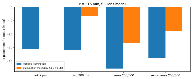
A source shifted by \(\delta\sigma = 0.084\) stops the mark from moving, but the other patterns keep 7 to 27 mrad: each pattern samples the pupil, and its decentred rim, differently, and an illumination tilt cannot undo a geometry error of the lens pupil for all of them. (The mark moves by 372 mrad per unit σ, less than the NA of 592 mrad that a pure tilt of the illumination would give: its edges are not formed by the zero order alone.) Illumination tuning suits what the illumination causes, the energetic telecentricity of section 4; the pupil centring has to be right in the lens (the stop position and the pupil aberrations of the design).

Summary

• The chief ray of Caldwell’s lens (stop on surface 30) is telecentric to 1.5 mrad across a 21 × 5 mm slit.

• The energetic telecentricity of the illumination adds up to about 1 mrad (conventional σ 0.8 and annular 0.8/0.5) from the coatings and the absorption, with a sign that depends on the coating design: outwards for the bare lens, inwards for single layers and most for the LaF\(_3\)/MgF\(_2\) V coat. The coating is part of the telecentricity budget.

• The pupil is decentred off axis by up to 5 % of its radius (pupil coma; it depends on where the stop is, which the paper does not say). A symmetric illumination does not see it, but every edge diffracts light to the rim, and the lithography simulation with the real pupil (lens_apodization()) shows pattern shifts through focus of 20–36 mrad at the slit edge, 30–46 mrad with the lens aberrations, different for each pattern.

• Scanning averages the \(x\) slopes over the slit height and turns the \(y\) slopes into image fading through focus.

• Tilting the illumination fixes one pattern (e.g. the marks) but not all of them: what is pattern dependent must be corrected in the lens.

Exercises: put the stop of the model on surface 31 (insert a plane surface or move stop_index) and repeat sections 3 and 6; add a radial thickness profile to the coatings (coatings.RadialProfile, thinner towards the rim of steep surfaces) and see how the energetic telecentricity changes; try a dipole illumination with fill= and Illumination.dipole.

print(f"run time {time.time() - t_start:.0f} s")

run time 302 s

References

• H. J. Levinson, Principles of Lithography, 4th ed., SPIE Press (2019).

• C. Mack, Fundamental Principles of Optical Lithography: The Science of Microfabrication, Wiley (2007).

• W. J. Smith, Modern Optical Engineering, 4th ed., McGraw-Hill (2008).

• J. B. Caldwell, “All-fused-silica 248-nm lithographic projection lens”, Optics & Photonics News 9(11), 40-41 (1998).