Jones pupils: polarization of the projection lens

A scalar pupil describes a projection lens by an amplitude (apodization) and a phase (wavefront, Zernikes). At high NA the lens also changes the polarization of the light: coatings and the Fresnel transmission of every surface treat s and p differently, and the glass can be birefringent (stress, or the intrinsic birefringence of CaF\(_2\)). The full description is the Jones pupil: a \(2\times 2\) complex matrix \(J(P_x, P_y)\) at every pupil point that maps the Jones vector of a ray entering the lens to the one leaving it.

Eight real functions over the pupil are hard to read and hard to specify. The literature uses these representations:

representation	idea	reference
Jones–Zernike	each element \(J_{jk}\) expanded into Zernikes	e.g. Totzeck et al. 2005
Pauli–Zernike	\(J = \sum_k a_k\sigma_k\), each \(a_k\) expanded into Zernikes; \(a_0\) is the scalar pupil, \(a_1, a_2\) linear and \(a_3\) circular retardance (imaginary parts) and diattenuation (real parts)	McIntyre, Kye, Levinson, Neureuther, JM3 5(3) 033001 (2006)
physical decomposition	polar decomposition \(J = \sqrt{T}e^{i\Phi}\,U H\): transmission, phase, retarder \(U\), diattenuator \(H\)	Totzeck, Gräupner, Heil et al., JM3 4(3) 031108 (2005); Geh et al.
orientation Zernike polynomials (OZP)	retardance and diattenuation are orientation fields (an axis, defined modulo 180°), expanded into vector polynomials with Zernike radial parts	Ruoff, Totzeck, JM3 8(3) 031404 (2009); US patent 8,126,669

McIntyre et al. found the Pauli form the most useful for lithographers: its coefficients separate the physical effects and are linear in small perturbations. The OZPs go one step further for retardance and diattenuation: like scalar Zernikes they sort the orientation fields by symmetry, so a rotationally symmetric radial retardance (typical for coatings and mount stress) is a single term, and they are used to specify and tolerance lenses through linear and quadratic sensitivities of CD and placement.

pyoptics.litho.jones_pupil implements these bases in a modular way:

• pauli_matrix, pauli_coefficients: the Pauli algebra,

• orientation_zernike(±j, P_x, P_y): OZPs as complex orientators \(o_1 + i o_2 = |o|e^{2i\psi}\),

• PauliZernikePupil, PhysicalJonesPupil (retardance and diattenuation in OZPs, circular parts in Zernikes), both with .fit() to sampled Jones matrices,

• compose/decompose: the polar decomposition.

Any callable J(P_x, P_y) can be passed as Projector(jones_pupil=...). It acts on the Jones vector of every diffraction order before the aplanatic rotation into image space, in Abbe and in Hopkins (hopkins.TCC) imaging. lens.lens_jones_pupil() computes the Jones pupil of a ray traced lens by polarization ray tracing (Chipman’s \(3\times 3\) matrices, Fresnel coefficients of each surface, optional thin film coatings).

About the lens. The ray traced example is the dioptric ArF water immersion lens of Zeiss patent US 7,187,503 B2 (raytrace.zeiss_arfi_lens(): 193.368 nm, NA 1.35, 8x, all fused silica, 11 aspheres, 1 mm of water in front of the wafer). Its rays reach the large angles of a hyper-NA lens, up to 65° in the water and on the last surfaces, which is where polarization effects come from. Production ArFi lenses are catadioptric and have optimized multilayer coatings; the quarter wave coatings and the CaF\(_2\) elements here are models of the mechanisms. Section 6 works with OZP coefficients chosen by hand on a generic ArF immersion Projector.

Contents:

1. Orientation Zernike polynomials.

2. Polarization ray trace of the ArFi lens: uncoated and with an antireflection coating.

3. The same Jones pupil in the Pauli–Zernike and OZP bases.

4. Where retardance comes from: coatings at large angles, the intrinsic birefringence of CaF\(_2\) and its compensation by clocking, stress.

5. Imaging with the lens Jones pupils at NA 1.35, with the coated lens and its CaF\(_2\) variants.

6. OZP sensitivities of CD at NA 1.35: what a lens specification needs.

import numpy as np
import matplotlib.pyplot as plt

from pyoptics.litho import Illumination, LithoSimulation, MaskLayout, Projector, ThinMask, lens
from pyoptics.litho import jones_pupil as jp
from pyoptics.litho.plot import plot_orientation
from pyoptics.raytrace import SIO2_ARF, WATER_ARF, zeiss_arfi_lens

plt.rcParams.update({"figure.dpi": 100, "font.size": 11})

1. Orientation Zernike polynomials

An orientation \(\psi\) (the fast axis of a retarder, the axis of best transmission of a diattenuator) is defined modulo 180°. It is described by the orientator \(o = |o|\,e^{2i\psi}\), a 2-vector that turns twice as fast as the axis. OZPs are a complete basis of orientator fields: the Zernike radial polynomials \(R_n^{|m|}(\rho)\) times \(e^{\pm i m\phi}\), real and imaginary (two OZPs per Zernike). Here they are labelled \(\pm j\) with the Fringe index \(j\) such that the first component of OZ \(+j\) is \(Z_j\), as in the patent; OZ \(-j\) flips the sign of the second component. Examples:

• OZ \(\pm 1\): constant orientation along x/y and along ±45°,

• OZ \(\pm 2\), \(\pm 3\): tilt-like, linear in \(\rho\),

• OZ \(+5 = \rho^2 e^{2i\phi}\): radial orientation (tangential for a negative coefficient), OZ \(-6\): the same rotated by 45°, a spiral; both are rotationally symmetric,

• OZ \(+4\), \(+9\): x/y orientation with defocus- and spherical-like radial dependence.

The plots show the magnitude (color) and the orientation (ticks).

terms = [1, -1, 2, -2, 4, 5, -5, -6, 7, -7, 9, 12]
fig, axes = plt.subplots(2, 6, figsize=(15, 5.4))
for ax, oz in zip(axes.ravel(), terms):
    plot_orientation(lambda P_x, P_y: jp.orientation_zernike(oz, P_x, P_y), ax=ax,
                     title="OZ {:+d}".format(oz), colorbar=False)
plt.tight_layout()

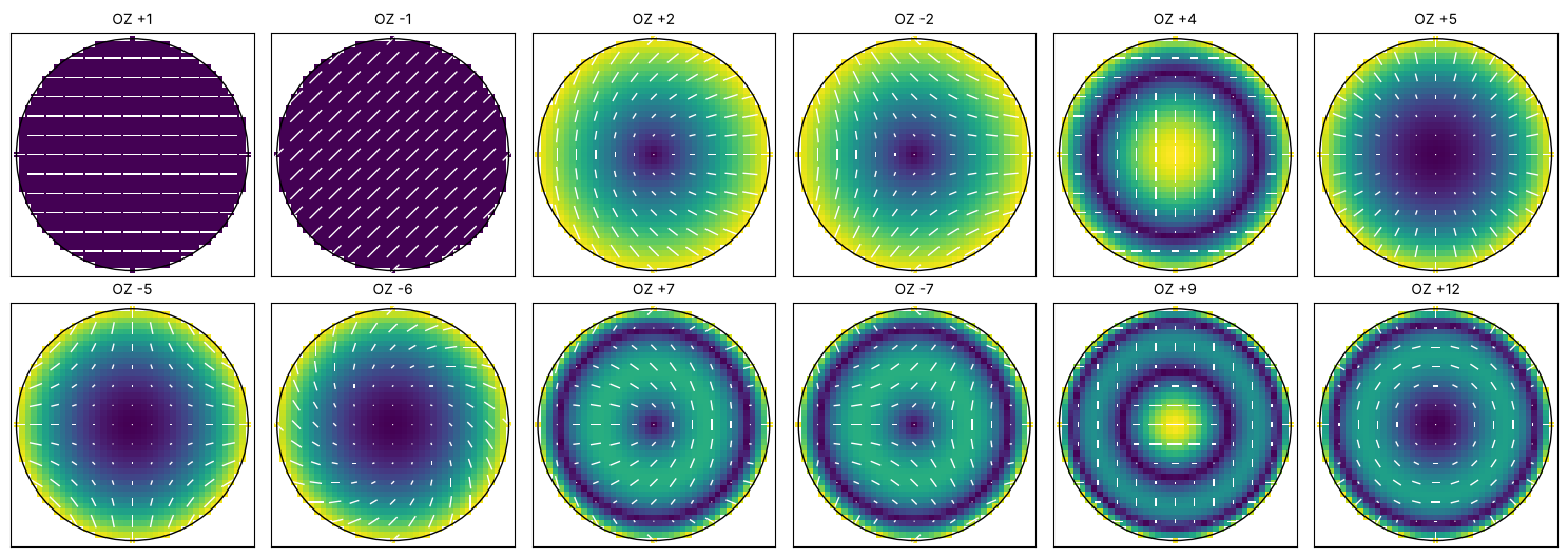
Under a rotation of the lens by \(\alpha\) an orientator rotates by \(2\alpha\), so the term \(e^{im\phi}\) picks up \(e^{i(2-m)\alpha}\). Only \(m = 2\) (\(+5\), \(-6\), \(+12\), \(-13\), …) is rotationally symmetric. This is why a rotationally symmetric lens has a Jones pupil of OZ \(+5, +12, +21, \dots\) (radial/tangential) and \(-6, -13, \dots\) (spiral) only, just as its wavefront has only \(Z_4, Z_9, \dots\).

2. Polarization ray trace of the ArFi lens

lens_jones_pupil() traces rays through the pupil of the water immersion lens (NA 1.35, 43 surfaces, see the introduction). At every surface it builds Chipman’s polarization ray tracing matrix

\[P = t_s\,\hat s\hat s^T + t_p\,\hat p'\hat p^T + \hat k'\hat k^T,\]

with the Fresnel amplitude transmissions \(t_s\), \(t_p\) (scaled such that \(|P\vec E|^2\) is the transmitted power) and multiplies them. The Jones pupil is the product between the aplanatic bases of the object and the image space ray (the identity for an ideal lens). It is normalized to the chief ray, which leaves the dose unchanged.

Two cases: uncoated (every surface reflects about 5 % at normal incidence), and every glass–helium surface with an ideal single-layer quarter-wave antireflection coating (\(n_c = \sqrt{n_\mathrm{glass}}\)). The last surface, glass to water, reflects only 0.3 % and stays bare.

system = zeiss_arfi_lens()
n_glass = SIO2_ARF
layers = lens.quarter_wave_coating(n_glass, system.wavelength)
last = len(system.surfaces) - 1  # glass to water

def coating(i, n):
    return None if i == last else layers

print("fused silica n = {:.4f}, coating n = {:.4f}, thickness {:.1f} nm".format(
    n_glass, layers[0][0], layers[0][1]*1e6))

uncoated = lens.lens_jones_pupil(system, N=41)
coated = lens.lens_jones_pupil(system, N=41, coating=coating)
for name, r in (("uncoated", uncoated), ("coated", coated)):
    print("{:9s}: chief ray transmission {:.3f}, {} rays, NA {:.3f}".format(
        name, r.transmission, len(r.P_x), r.NA))

fused silica n = 1.5608, coating n = 1.2493, thickness 38.7 nm

uncoated : chief ray transmission 0.133, 1257 rays, NA 1.350
coated   : chief ray transmission 0.998, 1257 rays, NA 1.350

decompose() splits every Jones matrix into the scalar transmission \(T\) and phase \(\Phi\), the linear diattenuation \(d\) (orientator, magnitude \((T_\max - T_\min)/(T_\max + T_\min)\)) and the linear retardance (orientator, in waves).

fig, axes = plt.subplots(2, 4, figsize=(16, 7.2))
for row, (name, r) in zip(axes, (("uncoated", uncoated), ("AR coated", coated))):
    parts = jp.decompose(r.J)
    d, g = parts["diattenuation"], parts["retardance"]
    plot_orientation((r.P_x, r.P_y, d[0] + 1j*d[1]), ax=row[0], title=name + ": diattenuation")
    plot_orientation((r.P_x, r.P_y, g[0] + 1j*g[1]), ax=row[1],
                     title=name + ": retardance (waves)")
    for ax, v, title in ((row[2], parts["transmission"], "transmission T"),
                         (row[3], parts["phase"]/(2*np.pi), "scalar phase (waves)")):
        im = ax.tripcolor(r.P_x, r.P_y, v, shading="gouraud", cmap="viridis")
        ax.set_aspect("equal"), ax.set_xticks([]), ax.set_yticks([])
        ax.set_title(name + ": " + title, fontsize=10)
        plt.colorbar(im, ax=ax, shrink=0.8)
plt.tight_layout()

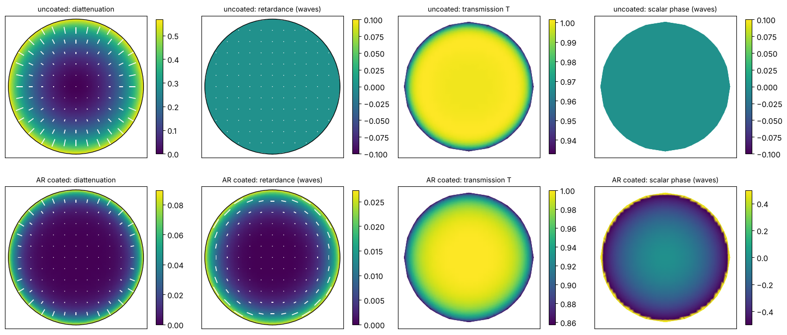
The uncoated lens is a pure radial diattenuator: \(p\) is transmitted better than \(s\) at oblique incidence (Brewster), and 43 surfaces add up to a strong effect at the rim of the pupil. The Fresnel coefficients are real, so there is no retardance. The coating removes most of the diattenuation but adds retardance, because the phase of the transmission of a thin film differs for s and p at oblique incidence. It also adds a rotationally symmetric scalar phase, a wavefront error that the lens designer has to include in the optimization.

3. The Jones pupil in the Pauli–Zernike and OZP bases

PauliZernikePupil.fit() expands the four Pauli coefficients into Zernikes, PhysicalJonesPupil.fit() the decomposition: OZPs for linear retardance and diattenuation, Zernikes for the circular parts and for the scalar transmission and phase (returned separately, since these belong to the Projector’s apodization and Zernikes).

def large(coefficients, tol=1e-4):
    return {k: round(v, 4) for k, v in coefficients.items() if abs(v) > tol}

fits = {}
for name, r in (("uncoated", uncoated), ("coated", coated)):
    physical, scalar = jp.PhysicalJonesPupil.fit(r.P_x, r.P_y, r.J, n_terms=25)
    pauli = jp.PauliZernikePupil.fit(r.P_x, r.P_y, r.J, n_terms=36)
    fits[name] = physical, scalar, pauli
    print(name)
    print("  diattenuation OZP:  ", large(physical.diattenuation))
    print("  retardance OZP:     ", large(physical.retardance))
    print("  circular retardance:", large(physical.circular_retardance))
    print("  scalar phase:       ", large(scalar["phase"]))
    print("  transmission:       ", large(scalar["transmission"]))
    print("  fit errors |J_fit - J|: physical {:.1e}, Pauli-Zernike {:.1e}".format(
        np.abs(jp.compose(*physical.fields(r.P_x, r.P_y)) - jp.scalar_free(r.J)).max(),
        np.abs(pauli(r.P_x, r.P_y) - r.J).max()))

uncoated
  diattenuation OZP:   {5: 0.4977, 12: 0.0557, 21: 0.0118}
  retardance OZP:      {}
  circular retardance: {}
  scalar phase:        {}
  transmission:        {1: 0.9944, 4: -0.0157, 9: -0.0187, 16: -0.0133, 17: 0.0002, 25: -0.0089}
  fit errors |J_fit - J|: physical 2.2e-03, Pauli-Zernike 1.8e-03
coated
  diattenuation OZP:   {5: 0.0441, 12: 0.0285, 21: 0.0128, -21: -0.0001}
  retardance OZP:      {5: -0.017, 12: -0.0079, 21: -0.0019}
  circular retardance: {}
  scalar phase:        {1: -0.1968, 4: -0.1088, 9: 0.2132, 16: 0.2555, 17: -0.0004, 25: 0.3765}
  transmission:        {1: 0.9731, 4: -0.0501, 9: -0.0342, 16: -0.0165, 17: 0.0002, 25: -0.0099}
  fit errors |J_fit - J|: physical 2.8e-03, Pauli-Zernike 7.2e-03

A handful of rotationally symmetric terms (OZ \(+5\), \(+12\), \(+21\)) describe the polarization of the centred lens. In the Pauli basis the same information is spread over \(a_1\) and \(a_2\), each with many Zernike terms:

physical, scalar, pauli = fits["coated"]
P = np.linspace(-1, 1, 81)
PX, PY = np.meshgrid(P, P)
a = pauli.pauli(PX, PY)
a = np.where(PX**2 + PY**2 <= 1, a, np.nan)
fig, axes = plt.subplots(2, 3, figsize=(12, 7))
for k in range(1, 4):
    for row, (part, f) in enumerate((("Re", np.real), ("Im", np.imag))):
        ax = axes[row, k - 1]
        v = f(a[k])
        lim = np.nanmax(np.abs(v)) or 1
        im = ax.pcolormesh(P, P, v, cmap="RdBu_r", vmin=-lim, vmax=lim, shading="auto")
        ax.set_aspect("equal"), ax.set_xticks([]), ax.set_yticks([])
        ax.set_title("{} $a_{}$".format(part, k), fontsize=10)
        plt.colorbar(im, ax=ax, shrink=0.8)
fig.suptitle("coated lens: Pauli coefficients (Re: diattenuation, Im: retardance)")
plt.tight_layout()

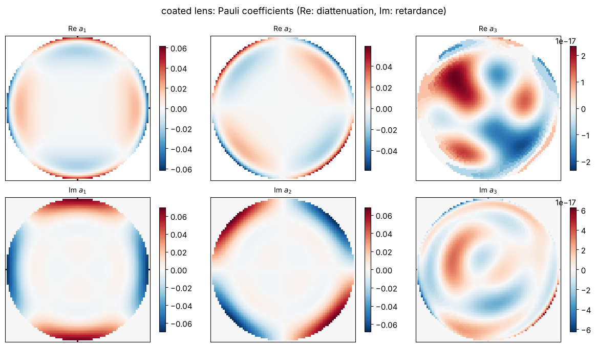
For a rotationally symmetric lens, \(a_1 \propto \cos 2\phi\) and \(a_2 \propto \sin 2\phi\) (astigmatism-like Zernikes \(Z_5, Z_6, Z_{12}, Z_{13}, \dots\)); the OZP basis collects both into one term per radial order.

Through the field

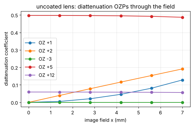
Off axis the chief ray crosses the lens surfaces obliquely. Constant (OZ \(\pm1\)) and tilt-like (OZ \(\pm2\), \(\pm3\)) terms appear, and they grow with the field, much like distortion and coma in the wavefront:

field_x = np.linspace(0, 7, 6)
rows = []
for x in field_x:
    r = lens.lens_jones_pupil(system, field=(x, 0.0), N=25)
    f, _ = jp.PhysicalJonesPupil.fit(r.P_x, r.P_y, r.J, n_terms=16)
    rows.append(f.diattenuation)
fig, ax = plt.subplots(figsize=(7, 4))
for oz in (1, 2, -3, 5, 12):
    ax.plot(field_x, [row[oz] for row in rows], "o-", label="OZ {:+d}".format(oz))
ax.set_xlabel("image field x (mm)"), ax.set_ylabel("diattenuation coefficient")
ax.set_title("uncoated lens: diattenuation OZPs through the field")
ax.legend(), ax.grid(alpha=0.3)

(<matplotlib.legend.Legend at 0x7f7473e5cec0>, None)

4. Where retardance comes from

The uncoated lens above is almost a pure diattenuator, because the Fresnel coefficients of a bare surface are real. Retardance, the phase difference between two polarizations, has other sources, and in practice it is the larger problem: it converts the TE polarization that a polarized illuminator delivers into TM, which images with less contrast at high NA (section 6).

• Coatings at large angles. A thin film shifts the phase of \(s\) and \(p\) differently as soon as the incidence is oblique. The difference grows quickly with the angle, so the surfaces near the wafer of a hyper-NA lens, with angles of incidence of 50–70°, dominate.

• Intrinsic birefringence of CaF\(_2\). ArF lenses use CaF\(_2\) for the elements that see the highest fluence (it does not compact like fused silica). As a cubic crystal it is isotropic to lowest order, but at short wavelengths it has a small birefringence that depends on the direction of the ray (Burnett et al. 2001): 3.4 nm/cm at 193 nm, 11.2 nm/cm at 157 nm. This was a main reason why 157 nm lithography was abandoned.

• Stress birefringence from mounts, from the annealing of large blanks and from compaction of fused silica under ArF exposure. It is specified in nm/cm and usually appears as low order radial or tangential OZ terms; PhysicalJonesPupil(retardance={5: ..., -6: ...}) models it directly.

Coatings: retardance per surface vs. the angle of incidence

One fused silica surface at 193.368 nm (\(n = 1.5608\)), uncoated and with the quarter wave coating of section 2, and the angles of incidence that occur on the surfaces of the lens (grey):

from pyoptics import thin_films

n_glass_arf = SIO2_ARF
wl_arf = system.wavelength_nm
layer = lens.quarter_wave_coating(n_glass_arf, wl_arf)[0]
angles = np.radians(np.linspace(0.0, 75.0, 151))

def surface_polarization(n_layer, d_layer):
    t = {pol: np.array([thin_films.r_t_coeffs(a, [n_layer], [0.0], [d_layer], 1.0, 0.0, n_glass_arf,
                                              0.0, pol, wl_arf)[1] for a in angles])
         for pol in ("s", "p")}
    T = {pol: np.array([thin_films.R_T_A_coeffs(a, [n_layer], [0.0], [d_layer], 1.0, 0.0, n_glass_arf,
                                                0.0, pol, wl_arf)[1] for a in angles])
         for pol in ("s", "p")}
    retardance = np.angle(t["p"]/t["s"])/(2*np.pi)  # waves
    return retardance, (T["p"] - T["s"])/(T["p"] + T["s"])

def max_angles_in_air(system, N=21):
    # largest angle of incidence on each surface, on the gas side (Snell), over the pupil and field
    n = system.n
    frames = system.frames()[0]
    p = np.linspace(-1, 1, N)
    PX, PY = np.meshgrid(p, p)
    inside = PX**2 + PY**2 <= 1
    worst = np.zeros(len(system.surfaces))
    for field in (0.0, system.max_field):
        b = system.trace_pupil(field, PX[inside], PY[inside])
        for i, s in enumerate(system.surfaces):
            o, R = frames[i]
            Q = (b.points[i + 1][b.valid] - o) @ R
            cos_i = np.abs(np.sum(s.normal(Q)*(b.directions[i][b.valid] @ R), axis=-1))
            worst[i] = max(worst[i], np.max(n[i]*np.sqrt(1 - cos_i**2)))
    return np.degrees(np.arcsin(np.clip(worst, 0, 1)))

aoi = max_angles_in_air(system)
fig, axes = plt.subplots(1, 2, figsize=(12, 4))
for (n_l, d_l), name in (((1.0, 0.0), "uncoated"), (layer, "quarter wave coating")):
    ret, dia = surface_polarization(n_l, d_l)
    axes[0].plot(np.degrees(angles), 1e3*ret, label=name)
    axes[1].plot(np.degrees(angles), dia, label=name)
axes[0].set_ylabel("retardance per surface (mwaves)"), axes[1].set_ylabel("diattenuation per surface")
for ax in axes:
    for a in aoi[1:-1]:
        ax.axvline(a, color="0.6", lw=0.6, alpha=0.6)
    ax.set_xlabel("angle of incidence in air (deg)"), ax.grid(alpha=0.3), ax.legend()
axes[0].set_title("193 nm, air to fused silica; grey: largest angle on each surface of the lens", fontsize=10)
plt.tight_layout()
gas = aoi[:-1]  # the glass to water surface has no gas side
print("surfaces with the largest angles (surface: deg):",
      ", ".join("{}: {:.0f}".format(system.surfaces[i].label, gas[i]) for i in np.argsort(gas)[::-1][:6]))

surfaces with the largest angles (surface: deg): 34: 68, 21: 66, 11: 51, 14: 48, 40: 47, 22: 46

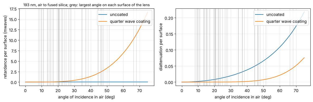
The uncoated surface has no retardance at all; the coating has some that grows steeply with the angle, and several surfaces of this lens see angles far beyond those of a dry lens. This is why ArFi lens coatings are designed for low retardance over the angles of each surface, and why a simple quarter wave coating, as used here, is only a teaching model.

Intrinsic birefringence of CaF\(_2\)

lens.CubicCrystal(delta_n, axis, clocking) adds this birefringence to the paths inside chosen elements of the ray trace. To lowest order the change of the index for a ray along \(\hat k\) (crystal axes) is set by the tensor \(\mathrm{diag}(k_x^2, k_y^2, k_z^2)\) on the transverse plane: it vanishes along the \(\langle 100\rangle\) and \(\langle 111\rangle\) axes and is largest along \(\langle 110\rangle\), where it equals \(\Delta n\). An element cut with [111] along the lens axis therefore has no retardance on axis, and a retardance with threefold symmetry for oblique rays; [100] elements have fourfold symmetry.

Production ArFi lenses use CaF\(_2\) for the last elements, where the fluence is highest. We make the last three elements of the lens “CaF\(_2\)” (the media behind surfaces 39, 41 and 43 of the patent, system indices 38, 40 and 42, 61, 54 and 60 mm thick) by giving them the birefringence of CaF\(_2\), keeping the fused silica index so that the design stays corrected. The surfaces carry the quarter wave coating.

DN_ARF = -3.4e-7  # CaF2 at 193 nm, Burnett et al. (2001)
dn = DN_ARF
caf2 = (38, 40, 42)

def crystal_pupil(axes_clockings, N=33):
    media = {i: lens.CubicCrystal(dn, a, np.radians(c)) for i, (a, c) in zip(caf2, axes_clockings)}
    return lens.lens_jones_pupil(system, N=N, coating=coating, birefringent=media)

def retardance_orientator(r):
    g = jp.decompose(r.J)["retardance"]
    return g[0] + 1j*g[1]

fig, axes = plt.subplots(1, 3, figsize=(15, 4.3))
r_si = coated
plot_orientation((r_si.P_x, r_si.P_y, retardance_orientator(r_si)), ax=axes[0],
                 title="fused silica (coating only)", label="retardance (waves)")
for ax, axis in zip(axes[1:], ("111", "100")):
    media = {42: lens.CubicCrystal(dn, axis)}
    r = lens.lens_jones_pupil(system, N=33, coating=coating, birefringent=media)
    plot_orientation((r.P_x, r.P_y, retardance_orientator(r)), ax=ax,
                     title="last element (60 mm) in CaF$_2$ [{}]".format(axis), label="retardance (waves)")
plt.tight_layout()

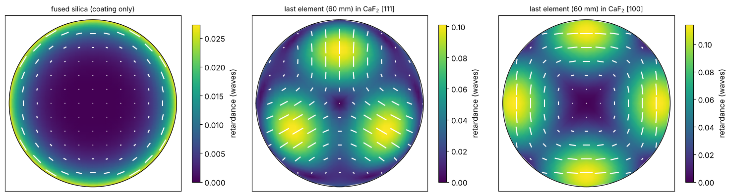
A single thick [111] element already brings a retardance of about a tenth of a wave at the rim, much more than the coatings, with a threefold pattern (OZ \(\pm3\), \(\pm8\), …: the terms that pick up \(e^{3i\alpha}\) under a rotation) on top of a rotationally symmetric part (OZ \(+5\)). The [100] element has a fourfold pattern (OZ \(-5\), …) and a rotationally symmetric part of the opposite sign.

Compensation by clocking

Rotating an element about the lens axis (clocking) rotates its pattern. Two [111] elements clocked by 60° have opposite threefold parts, which cancel as far as their paths are similar, and their rotationally symmetric parts add up; a [100] element can then compensate the rotationally symmetric part. This is the compensation that Burnett and coworkers proposed for the CaF\(_2\) elements of ArF and F\(_2\) lenses. Here we try all combinations of [111] at 0° or 60° and [100] at 0° or 45° for the three elements and rank them by the RMS retardance over the pupil:

import itertools

options = [("111", 0), ("111", 60), ("100", 0), ("100", 45)]
ranking = []
for combo in itertools.product(options, repeat=3):
    g = retardance_orientator(crystal_pupil(combo, N=21))
    ranking.append((np.sqrt(np.mean(np.abs(g)**2)), np.abs(g).max(), combo))
ranking.sort(key=lambda row: row[0])
print("RMS / max retardance (waves at 193 nm)   elements 39, 41, 43 (axis, clocking)")
for rms, peak, combo in ranking[:4] + ranking[-3:]:
    print("{:8.4f} {:8.4f}   {}".format(rms, peak, ", ".join("[{}] {:>2d}°".format(a, c) for a, c in combo)))
print("all [111], not clocked: RMS {:.4f}".format(next(rms for rms, _, c in ranking if c == (("111", 0),)*3)))
print("fused silica only: RMS {:.4f}".format(np.sqrt(np.mean(np.abs(retardance_orientator(coated))**2))))

unclocked, best = (("111", 0),)*3, ranking[0][2]
crystal = {"all [111], not clocked": crystal_pupil(unclocked), "best clocking": crystal_pupil(best)}
fig, axes = plt.subplots(1, 2, figsize=(10, 4.3))
vmax = max(np.abs(retardance_orientator(r)).max() for r in crystal.values())
for ax, (name, r) in zip(axes, crystal.items()):
    plot_orientation((r.P_x, r.P_y, retardance_orientator(r)), ax=ax, title=name, scale=vmax,
                     label="retardance (waves)")
plt.tight_layout()
for name, r in crystal.items():
    f, _ = jp.PhysicalJonesPupil.fit(r.P_x, r.P_y, r.J, n_terms=25)
    print(name, "retardance OZP:", large(f.retardance, 3e-3))

RMS / max retardance (waves at 193 nm)   elements 39, 41, 43 (axis, clocking)
  0.0275   0.0552   [111] 60°, [100]  0°, [111]  0°
  0.0275   0.0552   [111]  0°, [100]  0°, [111] 60°
  0.0279   0.0597   [111]  0°, [100] 45°, [111] 60°
  0.0279   0.0597   [111] 60°, [100] 45°, [111]  0°
  0.1095   0.1683   [100]  0°, [100] 45°, [100] 45°
  0.1101   0.1761   [100]  0°, [100]  0°, [100]  0°
  0.1121   0.1760   [100] 45°, [100] 45°, [100] 45°
all [111], not clocked: RMS 0.1077
fused silica only: RMS 0.0143

all [111], not clocked retardance OZP: {3: -0.1316, 5: 0.0738, 8: 0.1052, 12: -0.0617, 21: -0.0043}
best clocking retardance OZP: {3: -0.0197, 5: 0.004, -5: -0.0175, 8: 0.0372, 12: -0.0266, -12: 0.0062, 15: -0.0068}

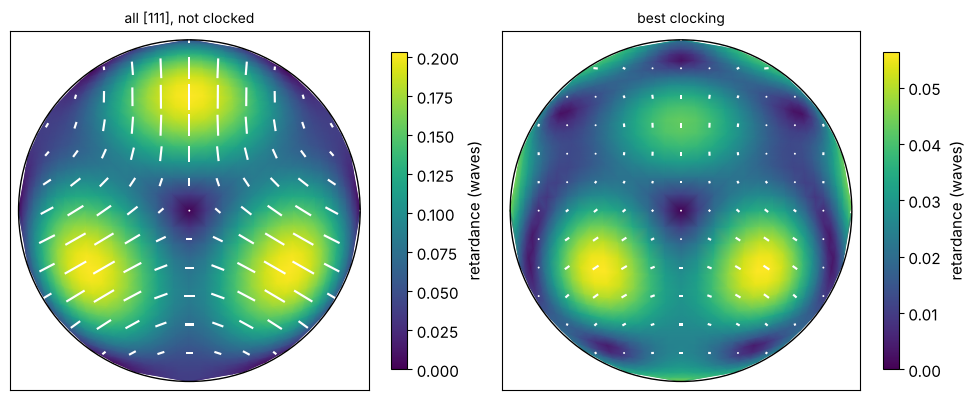
Clocking reduces the RMS retardance about fourfold (0.108 to 0.028 waves). What is left is mostly the part that the three elements of different thicknesses and ray angles cannot cancel; a real design chooses thicknesses and crystal axes together with the clocking, and adds compensating coatings or stress plates.

5. Imaging with the lens Jones pupils

Projector(jones_pupil=...) takes any of the fitted pupils. For the ArFi lens (NA 1.35, water) we compare the CD of dense lines through pitch with an annular source, polarized along x (TM for these vertical lines), along y (TE) and unpolarized. For the coated lens we use the polarization part only (PhysicalJonesPupil, without its scalar phase) and the full Jones pupil, which includes the coating’s wavefront.

uncoated_pupil = fits["uncoated"][2]  # Pauli-Zernike: the full Jones pupil
coated_full = fits["coated"][2]
coated_polarization = fits["coated"][0]  # retardance and diattenuation only
projector = Projector(uncoated.NA, system.wavelength_nm, n=WATER_ARF, magnification=8.0)
pupils = {"no Jones pupil": None, "uncoated": uncoated_pupil,
          "coated (polarization)": coated_polarization, "coated (full)": coated_full}
pitches = [90.0, 120.0, 180.0, 300.0]
sources = {pol: Illumination.annular(0.85, 0.55, n_samples=21, polarization=pol)
           for pol in ("x", "y", "unpolarized")}

cd = {}
for pol, source in sources.items():
    for name, pupil in pupils.items():
        cd[pol, name] = [LithoSimulation(MaskLayout.lines_spaces(p, p/2), ThinMask.binary(), source,
                                         projector.with_(jones_pupil=pupil)).cd(0.3)
                         for p in pitches]

fig, axes = plt.subplots(1, 3, figsize=(15, 4), sharey=True)
for ax, pol in zip(axes, sources):
    for name in list(pupils)[1:]:
        ax.plot(pitches, np.subtract(cd[pol, name], cd[pol, "no Jones pupil"]), "o-", label=name)
    ax.axhline(0, color="k", lw=0.8)
    ax.set_title("source polarization: " + pol, fontsize=10)
    ax.set_xlabel("pitch (nm)"), ax.grid(alpha=0.3)
axes[0].set_ylabel(r"$\Delta$CD vs. no Jones pupil (nm)")
axes[0].legend(fontsize=9)
plt.tight_layout()
print("CD change vs. no Jones pupil (nm), pitches", pitches)
for pol in sources:
    for name in list(pupils)[1:]:
        print("  {:12s} {:22s}".format(pol, name), np.round(np.subtract(cd[pol, name], cd[pol, "no Jones pupil"]), 2))

CD change vs. no Jones pupil (nm), pitches [90.0, 120.0, 180.0, 300.0]
  x            uncoated               [  nan -6.11 -0.75 -3.79]
  x            coated (polarization)  [  nan -0.41 -0.13 -0.36]
  x            coated (full)          [   nan  -6.91 -18.49 -25.15]
  y            uncoated               [ 8.15  1.37 -0.18  0.94]
  y            coated (polarization)  [0.59 0.09 0.   0.13]
  y            coated (full)          [  8.45  -2.16 -12.19 -15.11]
  unpolarized  uncoated               [ 7.57 -0.34 -0.2  -0.66]
  unpolarized  coated (polarization)  [ 0.27 -0.02 -0.04 -0.06]
  unpolarized  coated (full)          [ 19.72  -3.38 -15.01 -19.38]

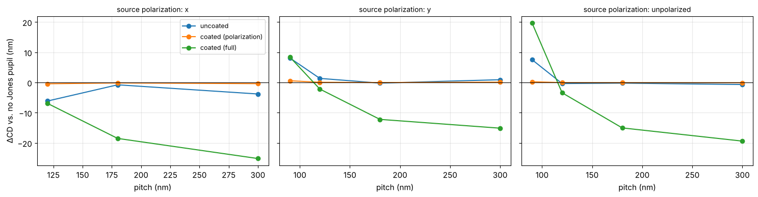
The radial diattenuation of the uncoated lens favours the TM (\(p\)) part of the orders at the rim of the pupil. At NA 1.35 the first orders of the densest pitch pass close to the rim, so it changes the balance between the orders and with it the CD: by 8 nm at a pitch of 90 nm with y (TE) polarization, and by 6 nm at 120 nm with x (TM) polarization (at 90 nm the TM image is too weak to print). With unpolarized light the TE part dominates the image of the densest pitch, and the shift stays. The polarization part of the coated lens moves the CD by less than 1 nm. Its scalar phase, however, is a rotationally symmetric wavefront of several tenths of a wave (\(Z_9\), \(Z_{16}\), \(Z_{25}\): the quarter wave coatings at the steep surfaces near the wafer) and changes the CD of the larger pitches by up to 25 nm: for a real lens it is part of the wavefront budget and is designed out together with the coatings.

The CaF\(_2\) variants

The case for the retardance of section 4: 45 nm lines and spaces, vertical (V) and horizontal (H), with a dipole across the lines, TE polarized and unpolarized, imaged with the polarization part of the coated lens and its CaF\(_2\) variants.

arfi = projector
variants = {"fused silica (coated)": coated, **crystal}
variant_pupils = {name: jp.PhysicalJonesPupil.fit(r.P_x, r.P_y, r.J, n_terms=36)[0]
                  for name, r in variants.items()}

def lines_sim(orientation, polarization):
    dipole_axis = "x" if orientation == "y" else "y"
    return LithoSimulation(MaskLayout.lines_spaces(90.0, 45.0, orientation=orientation), ThinMask.binary(),
                           Illumination.dipole(0.9, 0.6, axis=dipole_axis, n_samples=15,
                                               polarization=polarization), arfi)

print("{:28s} {:>22s} {:>22s} {:>22s}".format("", "TE dipole, V lines", "TE dipole, H lines",
                                              "unpolarized: CD H - V"))
for name, pupil in [("no Jones pupil", None)] + list(variant_pupils.items()):
    row = []
    for orientation, pol in (("y", "y"), ("x", "x")):
        s = lines_sim(orientation, pol)
        s = s.with_(projector=arfi.with_(jones_pupil=pupil))
        row.append("CD {:5.2f}, NILS {:5.3f}".format(s.cd(0.3), s.nils(0.3)))
    cds = [lines_sim(o, "unpolarized").with_(projector=arfi.with_(jones_pupil=pupil)).cd(0.3) for o in ("y", "x")]
    print("{:28s} {:>22s} {:>22s} {:>19.2f} nm".format(name, *row, cds[1] - cds[0]))

                                 TE dipole, V lines     TE dipole, H lines  unpolarized: CD H - V
no Jones pupil                 CD 40.04, NILS 2.940   CD 40.04, NILS 2.940                0.00 nm
fused silica (coated)          CD 40.07, NILS 2.941   CD 40.07, NILS 2.941                0.00 nm
all [111], not clocked         CD 39.55, NILS 2.619   CD 40.05, NILS 2.925                5.07 nm

best clocking                  CD 40.05, NILS 2.929   CD 40.06, NILS 2.936                0.09 nm

With TE polarized dipoles the unclocked CaF\(_2\) elements cost about 11 % of the NILS on the vertical lines, while the horizontal lines barely notice: the threefold retardance pattern is not the same along x and y in the pupil, so the loss of TE polarization depends on the orientation of the feature. With unpolarized light the same pattern shows up as an H–V CD difference of 5 nm. The best clocking removes almost all of it, although its RMS retardance is only four times smaller: the residual retardance has its axes along x and y where the dipole poles sit (radial, tangential and the fourfold [100] pattern), and there the TE light is an eigenpolarization that a retarder leaves alone. What matters is not the size of the retardance alone, but its orientation relative to the polarization at the pupil positions the illumination uses. This is the kind of result that drives the retardance specification of ArFi lenses.

6. OZP sensitivities at NA 1.35

This section does not use the ray traced lens: it applies single OZP terms, chosen by hand, to a generic ArF immersion projector. At immersion NA the angles in the resist are large, so polarization matters most. As for Zernikes (notebook 33) the response of a CD (or of the NILS) to an OZP coefficient \(c\) is the expansion

\[\Delta\mathrm{CD} = \frac{\partial\,\mathrm{CD}}{\partial c}\,c + \frac{1}{2}\frac{\partial^2\mathrm{CD}}{\partial c^2}\,c^2 .\]

Evaluating each OZP at \(+c\) and \(-c\) separates the two parts: a linear response flips its sign, a quadratic one does not. The case: 45 nm lines and spaces, a y-polarized (TE) dipole, ArF water immersion; retardance \(c = 0.02\) waves, diattenuation \(c = 0.05\).

immersion = Projector(1.35, 193.0, n=1.437)
sim = LithoSimulation(MaskLayout.lines_spaces(90.0, 45.0), ThinMask.binary(),
                      Illumination.dipole(0.9, 0.6, n_samples=15, polarization="y"), immersion)
cd0, nils0 = sim.cd(0.3), sim.nils(0.3)
print("without Jones pupil: CD {:.2f} nm, NILS {:.3f}".format(cd0, nils0))

def response(kind, oz, value):
    s = sim.with_(projector=immersion.with_(jones_pupil=jp.PhysicalJonesPupil(**{kind: {oz: value}})))
    return s.cd(0.3) - cd0, s.nils(0.3) - nils0

terms = jp.oz_indices(9)
deltas = {"retardance": 0.02, "diattenuation": 0.05}
results = {(kind, sign): np.array([response(kind, oz, sign*delta) for oz in terms])
           for kind, delta in deltas.items() for sign in (1, -1)}

fig, axes = plt.subplots(2, 2, figsize=(15, 6.5), sharex=True)
x = np.arange(len(terms))
for row, (kind, delta) in zip(axes, deltas.items()):
    for col, metric in enumerate((r"$\Delta$CD (nm)", r"$\Delta$NILS")):
        ax = row[col]
        for sign, offset in ((1, -0.2), (-1, 0.2)):
            ax.bar(x + offset, results[kind, sign][:, col], 0.4, label="c = {:+g}".format(sign*delta))
        ax.axhline(0, color="k", lw=0.8)
        ax.set_ylabel(metric), ax.grid(alpha=0.3)
        ax.set_title(kind, fontsize=10)
        ax.legend(fontsize=9)
for ax in axes[1]:
    ax.set_xticks(x), ax.set_xticklabels(["{:+d}".format(t) for t in terms], fontsize=9)
    ax.set_xlabel("OZ index")
plt.tight_layout()

without Jones pupil: CD 40.08 nm, NILS 2.936

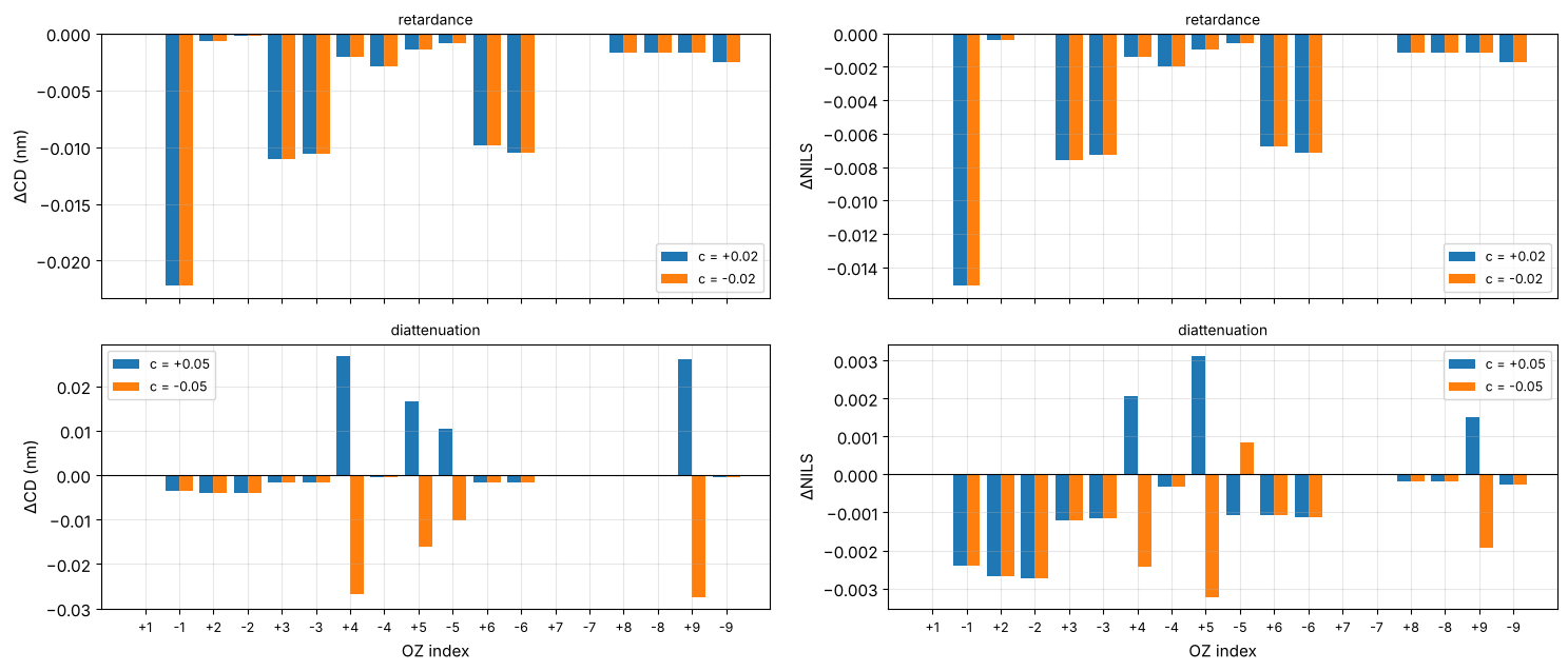
Two classes of response appear, in line with the sensitivity analysis of Ruoff and Totzeck:

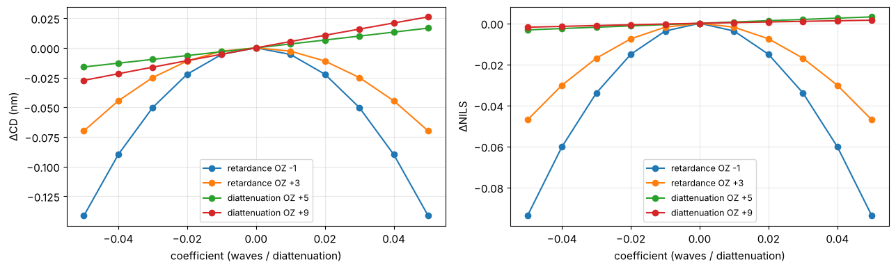
• Retardance acts quadratically: both signs lower the NILS by the same amount. The TE light at the poles is an eigenstate of an x/y retarder (OZ \(+1\) does nothing), but any other orientation converts part of it into TM light, which images with less contrast at this NA. OZ \(-1\) (45°) is the most harmful; the other terms matter as far as they rotate the axis at the positions of the orders in the pupil.

• Diattenuation acts linearly through the terms that change the transmission of the zero order relative to the first orders, which lie at different positions in the pupil (OZ \(+4\), \(\pm5\), \(+9\) here). A constant x/y term (OZ \(+1\)) only scales the dose, which the normalization to the open frame removes.

A tolerance therefore follows from the quadratic coefficient for retardance and from the linear one for diattenuation. For this two-beam case the effects are small: even 0.05 waves of the worst retardance term (OZ \(-1\)) cost about 0.1 nm of CD and 3 % of the NILS.

c = np.linspace(-0.05, 0.05, 11)
fig, axes = plt.subplots(1, 2, figsize=(13, 4))
for kind, oz in (("retardance", -1), ("retardance", 3), ("diattenuation", 5), ("diattenuation", 9)):
    r = np.array([response(kind, oz, v) for v in c])
    for ax, col in zip(axes, r.T):
        ax.plot(c, col, "o-", label="{} OZ {:+d}".format(kind, oz))
for ax, label in zip(axes, (r"$\Delta$CD (nm)", r"$\Delta$NILS")):
    ax.set_xlabel("coefficient (waves / diattenuation)"), ax.set_ylabel(label)
    ax.grid(alpha=0.3), ax.legend(fontsize=9)
plt.tight_layout()

Summary

• jones_pupil: Pauli algebra, orientation Zernike polynomials, the polar decomposition and two fitted representations, PauliZernikePupil and PhysicalJonesPupil (OZP retardance and diattenuation). Both plug into Projector(jones_pupil=...) for Abbe and Hopkins imaging, and they can be chained with @.

• lens.lens_jones_pupil(): polarization ray trace of a lens with Fresnel coefficients, optional coatings (quarter_wave_coating() or any thin film stack per surface) and birefringent elements (CubicCrystal, the intrinsic birefringence of CaF\(_2\) with any axis and clocking).

• The ray traced lens is a published ArF water immersion design (NA 1.35); section 6 uses OZP terms chosen by hand on a generic ArFi projector.

• The uncoated lens is a strong radial diattenuator (OZ \(+5\)); a coating trades diattenuation for retardance and adds a scalar wavefront.

• Retardance comes from coatings at large angles, CaF\(_2\) elements and stress. CaF\(_2\) elements bring threefold ([111]) or fourfold ([100]) patterns that clocking largely compensates; uncompensated, they cost NILS with polarized illumination and cause an H–V bias at NA 1.35.

• OZPs sort polarization errors by symmetry like Zernikes sort wavefronts; CD responds quadratically to retardance and linearly to diattenuation.

• Not included: a ray traced stress birefringence (modelled here by OZP terms), and polarization effects of the mask and resist interfaces beyond those already in FilmMask, RigorousMask and WaferStack.

References

• G. R. McIntyre, J. Kye, H. Levinson and A. R. Neureuther, “Polarization aberrations in hyper-numerical-aperture projection printing: a comparison of various representations”, J. Micro/Nanolith. MEMS MOEMS 5, 033001 (2006).

• M. Totzeck, P. Gräupner, T. Heil et al., “Polarization influence on imaging”, J. Microlith. Microfab. Microsyst. 4, 031108 (2005).

• J. Ruoff and M. Totzeck, “Orientation Zernike polynomials: a useful way to describe the polarization effects of optical imaging systems”, J. Micro/Nanolith. MEMS MOEMS 8, 031404 (2009).

• S.-Y. Lu and R. A. Chipman, “Interpretation of Mueller matrices based on polar decomposition”, J. Opt. Soc. Am. A 13, 1106-1113 (1996).

• J. H. Burnett, Z. H. Levine and E. L. Shirley, “Intrinsic birefringence in calcium fluoride and barium fluoride”, Phys. Rev. B 64, 241102 (2001).

• G. Yun, K. Crabtree and R. A. Chipman, “Three-dimensional polarization ray-tracing calculus I: definition and diattenuation”, Appl. Opt. 50, 2855-2865 (2011).

• R. A. Chipman, W.-S. T. Lam and G. Young, Polarized Light and Optical Systems, CRC Press (2018).