Beam widths and M² after ISO 11146
pyoptics.beam_quality measures laser beams the way ISO 11146 prescribes:
Function |
Result |
|---|---|
|
centroid \((\bar x, \bar y)\) and second moments \(\sigma_x^2, \sigma_y^2, \sigma_{xy}^2\) of an intensity image |
|
widths \(d_x, d_y\) along the principal axes and their azimuth \(\varphi\), optionally with the iterative integration window of ISO 11146-3 |
|
hyperbolic fit \(d^2(z) = a + bz + cz^2\) giving waist \(d_0\), waist position \(z_0\), divergence \(\Theta\), Rayleigh length \(z_R\) and \(M^2\) |
The widths are second moment diameters, \(d_x = 2\sqrt2\,\bigl(\sigma_x^2 + \sigma_y^2 + \gamma\sqrt{(\sigma_x^2 - \sigma_y^2)^2 + 4\sigma_{xy}^4}\bigr)^{1/2}\) (and \(d_y\) with \(-\gamma\), \(\gamma = \operatorname{sgn}(\sigma_x^2 - \sigma_y^2)\)), which equal \(2w\) for a Gaussian beam with \(1/e^2\) radius \(w\). The beam propagation ratio is
1 for a Gaussian beam and \(2l + 1\) for a Hermite-Gaussian \(\mathrm{HG}_{lm}\) in \(x\).
Convention: \(\exp(i(\mathbf{k}\cdot\mathbf{r} - \omega t))\); lengths in µm.
import warnings

import numpy as np
import matplotlib.pyplot as plt
from matplotlib.patches import Ellipse

from pyoptics.beam_quality import beam_widths, fit_caustic
from pyoptics.bases import local_coordinates
from pyoptics.beams import gauss_hermite
from pyoptics.masks import thin_lens
from pyoptics.processing import CameraNoiser, Scaler
from pyoptics.propagators import rayleigh_sommerfeld_I_TF
from pyoptics.utils import grid2d

plt.rcParams.update({"figure.dpi": 100, "image.origin": "lower", "font.size": 11})
1. Widths, principal axes and azimuth
Three test beams: a round Gaussian, an elliptical Gaussian rotated by 30°,
and a Hermite-Gaussian \(\mathrm{HG}_{10}\) rotated by \(-20°\). The ellipses show
\(d_x, d_y\) and the principal axes found by beam_widths(). The principal
“x” axis is, by ISO’s definition, the one closer to the lab \(x\) axis
(\(\lvert\varphi\rvert \le 45°\)).
x, y, X, Y = grid2d(-150, 150, -150, 150, 300)
U, V = local_coordinates(X, Y, 20.0, -10.0, np.deg2rad(30))
U2, V2 = local_coordinates(X, Y, -15.0, 5.0, np.deg2rad(-20))
beams = {
    "Gaussian, w = 30 µm": np.exp(-2*(X**2 + Y**2)/30.0**2),
    "elliptical, 50 × 20 µm, 30°": np.exp(-2*(U**2/50.0**2 + V**2/20.0**2)),
    "HG$_{10}$, w = 25 µm, −20°": np.abs(gauss_hermite(1, 0, U2, V2, 0.0, 25.0, 1.0, 1.0))**2,
}

fig, axes = plt.subplots(1, 3, figsize=(15, 4.8))
for ax, (name, I) in zip(axes, beams.items()):
    b = beam_widths(I, x, y)
    ax.imshow(I, extent=(x[0], x[-1], y[0], y[-1]), cmap="magma")
    ax.add_patch(Ellipse((b.x_c, b.y_c), b.d_x, b.d_y, angle=np.rad2deg(b.phi), fill=False, color="c", lw=1.5))
    for d, ang in ((b.d_x, b.phi), (b.d_y, b.phi + np.pi/2)):
        ax.plot(b.x_c + d/2*np.cos(ang)*np.array([-1, 1]), b.y_c + d/2*np.sin(ang)*np.array([-1, 1]), "c--", lw=1)
    ax.set_title(f"{name}\n$d_x$ = {b.d_x:.1f}, $d_y$ = {b.d_y:.1f} µm, φ = {np.rad2deg(b.phi):.1f}°", fontsize=10)
    ax.set_xlabel("$x$ [µm]")
fig.tight_layout()
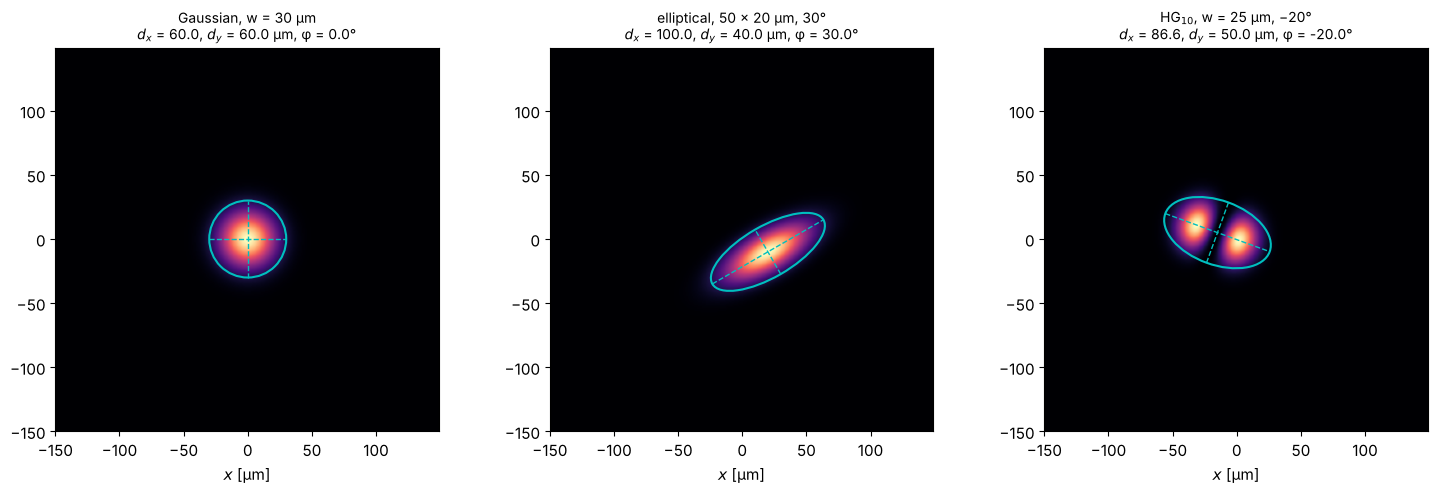
The numbers are exact: \(2w = 60\) µm for the round beam, \(100 \times 40\) µm for the ellipse, and \(2w\sqrt{3} = 86.6\) µm by \(2w = 50\) µm for \(\mathrm{HG}_{10}\), whose second moment width in \(x\) includes both lobes.
2. M² of a focused beam with spherical aberration
A collimated Gaussian beam (\(w = 100\) µm, λ = 1 µm) is focused by a lens with
\(f = 10\) mm. Spherical aberration is modelled as an additional pupil phase
\(2\pi a\,(r/w)^4\) with \(a\) in waves at \(r = w\). The field is propagated with the
angular spectrum method (rayleigh_sommerfeld_I_TF) and measured like in the
lab, in two steps as ISO recommends:
a coarse scan over a wide range to locate the waist and estimate \(z_R\),
the actual measurement: 5 positions within \(\pm z_R\) of the waist and 6 beyond \(2 z_R\).
Even the unaberrated beam shows a known Gaussian beam effect: its waist does not lie in the focal plane but at \(f/(1 + (f/z_{R,\mathrm{in}})^2) = 9.08\) mm, closer to the lens, because the input Rayleigh length \(z_{R,\mathrm{in}} = \pi w^2/\lambda = 31\) mm is not much longer than \(f\).
wl, w, f = 1.0, 100.0, 10000.0
x, y, X, Y = grid2d(-600, 600, -600, 600, 512)
R = np.hypot(X, Y)

def widths_along(E, z_positions):
    return [beam_widths(np.abs(rayleigh_sommerfeld_I_TF(E, x, y, z, wl)[0])**2, x, y) for z in z_positions]

def measure(E):
    z_coarse = np.linspace(4000, 16000, 13)
    coarse = fit_caustic(z_coarse, [b.d_x for b in widths_along(E, z_coarse)], wl)
    z_iso = coarse.z_0 + coarse.z_R*np.array([-3, -2.5, -2, -0.8, -0.4, 0, 0.4, 0.8, 2, 2.5, 3])
    d_iso = np.array([b.d_x for b in widths_along(E, z_iso)])
    return z_iso, d_iso, fit_caustic(z_iso, d_iso, wl)

aberrations = (0.0, 0.05, 0.1, 0.15)
results = {}
for a in aberrations:
    E_lens = np.exp(-R**2/w**2)*thin_lens(x, y, f, wl)*np.exp(2j*np.pi*a*(R/w)**4)
    results[a] = (E_lens,) + measure(E_lens)
    fit = results[a][3]
    print(f"a = {a:4.2f} waves:  M² = {fit.M2:.3f}, waist at {fit.z_0/1000:.2f} mm, "
          f"d_0 = {fit.d_0:.1f} µm, z_R = {fit.z_R/1000:.2f} mm, Θ = {1000*fit.theta:.2f} mrad")
a = 0.00 waves: M² = 1.000, waist at 9.08 mm, d_0 = 60.7 µm, z_R = 2.89 mm, Θ = 20.99 mrad
a = 0.05 waves: M² = 1.084, waist at 10.51 mm, d_0 = 79.0 µm, z_R = 4.52 mm, Θ = 17.48 mrad
a = 0.10 waves: M² = 1.255, waist at 11.21 mm, d_0 = 107.9 µm, z_R = 7.29 mm, Θ = 14.80 mrad
a = 0.15 waves: M² = 1.442, waist at 10.09 mm, d_0 = 139.8 µm, z_R = 10.65 mm, Θ = 13.13 mrad
fig, axes = plt.subplots(1, 2, figsize=(14, 4.8))
z_plot = np.linspace(-22000, 45000, 400)
for (a, (E, z_iso, d_iso, fit)), color in zip(results.items(), ("k", "C0", "C1", "C3")):
    axes[0].plot(z_iso/1000, d_iso/2, "o", color=color, ms=5)
    axes[0].plot(z_plot/1000, fit.d(z_plot)/2, "-", color=color, lw=1.5, label=f"a = {a}: M² = {fit.M2:.2f}")
axes[0].axvline(f/1000, color="gray", ls=":", lw=1)
axes[0].set_xlim(z_plot[0]/1000, z_plot[-1]/1000); axes[0].set_ylim(0, 250)
axes[0].set_xlabel("$z$ [mm]"); axes[0].set_ylabel("$d_x/2$ [µm]")
axes[0].set_title("ISO measurement positions (dots) and fitted caustics; dotted: focal plane", fontsize=10)
axes[0].legend(fontsize=9)

E, z_iso, d_iso, fit = results[0.15]
z_map = np.linspace(-22000, 45000, 81)
profiles = np.array([np.abs(rayleigh_sommerfeld_I_TF(E, x, y, z, wl)[0][256])**2 for z in z_map])
axes[1].imshow((profiles/profiles.max(axis=1, keepdims=True)).T**0.5, extent=(z_map[0]/1000, z_map[-1]/1000, x[0], x[-1]),
               aspect="auto", cmap="inferno")
axes[1].plot(z_map/1000, fit.d(z_map)/2, "c--", lw=1); axes[1].plot(z_map/1000, -fit.d(z_map)/2, "c--", lw=1)
axes[1].set_ylim(-400, 400); axes[1].set_xlabel("$z$ [mm]"); axes[1].set_ylabel("$x$ [µm]")
axes[1].set_title("a = 0.15: $\\sqrt{I(x, 0, z)}$, each $z$ normalized; dashed: $\\pm d_x/2$", fontsize=10)
fig.tight_layout()
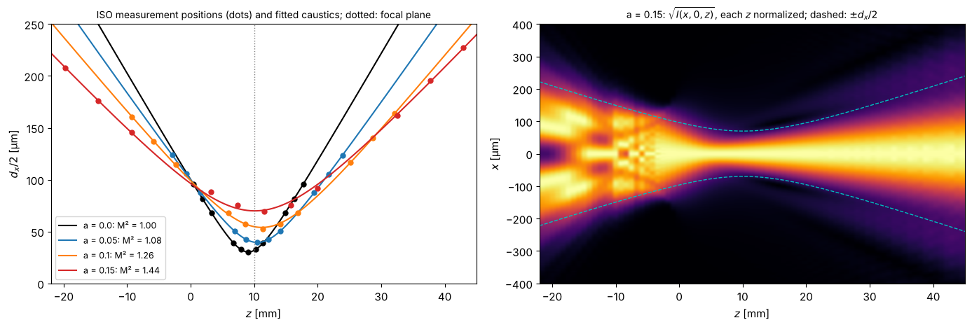
Spherical aberration moves the waist away from the lens and increases M²: the beam is no longer Gaussian, it converges and diverges faster than its waist allows for a Gaussian beam.
Cross-check: M² from a single plane
The second moments propagate exactly like a Gaussian beam’s, so M² can also be computed from the field in one plane, without any caustic: with the intensity weighted moments of position and propagation angle \(\theta_x = k_x/k\),
(centred moments). This needs the phase, so it works for simulations but not for camera images; it is a good check of the measurement procedure. The table compares it with caustic fits using the ISO window and using the moments of the whole (noise-free) image:
from pyoptics.fft import FT, inv_FT
from pyoptics.utils import freq_grid

def M2_from_field(E):
    k = 2*np.pi/wl
    K_X = freq_grid(x, y, wavenumbers=True)[0]
    I = np.abs(E)**2/np.sum(np.abs(E)**2)
    S = np.abs(FT(E))**2/np.sum(np.abs(FT(E))**2)
    dE_dx = inv_FT(1j*K_X*FT(E))   # spectral derivative, exact for band limited fields
    x_mean = np.sum(X*I)
    theta_mean = np.sum(K_X*S)/k
    x2 = np.sum((X - x_mean)**2*I)
    theta2 = np.sum((K_X/k - theta_mean)**2*S)
    x_theta = np.sum((X - x_mean)*np.imag(np.conj(E)*dE_dx))/np.sum(np.abs(E)**2)/k
    return 2*k*np.sqrt(x2*theta2 - x_theta**2)

print("              ISO (3x window)   whole image   single plane")
for a, (E, z_iso, d_iso, fit) in results.items():
    d_full = [beam_widths(np.abs(rayleigh_sommerfeld_I_TF(E, x, y, z, wl)[0])**2, x, y, iterate=False).d_x
              for z in z_iso]
    print(f"a = {a:4.2f}:  M² = {fit.M2:10.3f} {fit_caustic(z_iso, d_full, wl).M2:13.3f} {M2_from_field(E):14.3f}")
ISO (3x window) whole image single plane
a = 0.00: M² = 1.000 1.000 1.000
a = 0.05: M² = 1.084 1.094 1.094
a = 0.10: M² = 1.255 1.335 1.338
a = 0.15: M² = 1.442 1.626 1.666
Without aberrations all three agree. With spherical aberration, the whole image moments reproduce the single plane value (the small remaining difference at \(a = 0.15\) is light that leaves the 1.2 mm simulation window), but the ISO procedure gives a clearly smaller M²: the aberrated beam carries a faint halo far outside its core, which the 3 × window cuts off, and second moments weight exactly these far wings strongly. M² of non-Gaussian beams thus depends on the measurement convention; ISO’s window trades this bias for robustness against noise, as the next section shows.
3. Noise, background and the integration window
Second moments weight the intensity with the squared distance from the centroid, so noise and background far from the beam dominate them quickly. A camera image of a Gaussian beam (\(w = 12\) pixels on a 256 × 256 sensor) with shot noise, 5 e⁻ read noise and an offset of 100 DN illustrates the three rules of ISO 11146-3:
subtract the background (here from a dark frame),
restrict the integration to a window of 3 × the beam widths around the centroid,
iterate widths and window until they converge.
For each peak signal, 30 noisy frames are evaluated; the plot shows the rms deviation of \(d_x\) from the true 24 pixels (bias and scatter combined).
x, y, X, Y = grid2d(-128, 128, -128, 128, 256)   # pixel units
w_px = 12.0
beam = np.exp(-2*(X**2 + Y**2)/w_px**2)
camera = CameraNoiser(model="camera", read_noise=5.0, gain=1.0, offset=100.0, rng=1)
dark = np.mean([camera(np.zeros_like(beam)) for _ in range(20)], axis=0)

peaks = np.logspace(np.log10(200), 5, 7)
methods = {
    "no background subtraction, whole image": dict(background=0.0, iterate=False),
    "dark frame subtracted, whole image": dict(background=dark, iterate=False),
    "dark frame subtracted, ISO window (iterated)": dict(background=dark, iterate=True),
}
def width_or_nan(F, **kwargs):
    with warnings.catch_warnings(), np.errstate(invalid="ignore"):
        warnings.simplefilter("ignore")  # non-converged iterations at the lowest signals
        try:
            return beam_widths(F, x, y, **kwargs).d_x
        except ValueError:  # iteration failed: signal too low
            return np.nan

errors = {m: [] for m in methods}
for peak in peaks:
    frames = [camera(Scaler(peak)(beam)) for _ in range(30)]
    for m, kwargs in methods.items():
        d = np.array([width_or_nan(F, **kwargs) for F in frames])
        # nan: negative variances, the moments of the whole noisy image are undefined
        errors[m].append((np.nanmean(d)/(2*w_px) - 1, np.nanstd(d)/(2*w_px), np.mean(np.isnan(d))))

fig, axes = plt.subplots(1, 2, figsize=(14, 4.6))
for (m, err), color in zip(errors.items(), ("C3", "C1", "C0")):
    err = np.array(err)
    axes[0].loglog(peaks, 100*np.hypot(err[:, 0], err[:, 1]), "o-", color=color, label=m)
axes[0].set_xlabel("peak signal [photons/pixel]"); axes[0].set_ylabel("rms deviation of $d_x$ [%]")
axes[0].set_title("Width error vs. signal (bias and scatter of 30 frames)"); axes[0].legend(fontsize=8)

F = camera(Scaler(1000.0)(beam))
b = beam_widths(F, x, y, background=dark)
axes[1].imshow(F - dark, extent=(x[0], x[-1], y[0], y[-1]), cmap="magma", vmin=-20, vmax=200)
half = 1.5*b.d_r   # round beam (ellipticity > 0.87): square window aligned with x and y
axes[1].add_patch(plt.Rectangle((b.x_c - half, b.y_c - half), 2*half, 2*half, fill=False, color="c"))
axes[1].add_patch(Ellipse((b.x_c, b.y_c), b.d_x, b.d_y, angle=np.rad2deg(b.phi), fill=False, color="w", lw=1))
axes[1].set_title(f"1000 photons peak: $d_x$ = {b.d_x:.1f} px (true 24), cyan: ISO window")
axes[1].set_xlabel("$x$ [px]")
fig.tight_layout()
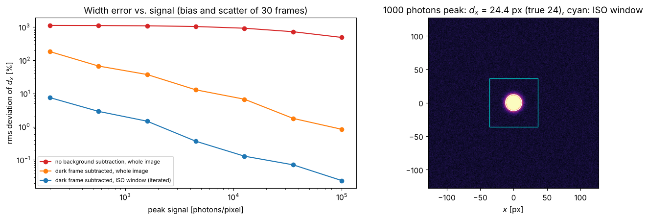
Without background subtraction the offset of 100 DN over the whole sensor makes the “width” meaningless (errors of several 100 %). Subtracting a dark frame removes the offset, but the noise of 65 000 pixels, weighted with their squared distance from the beam, still biases and scatters the result; at low signal the variances of the whole image can even become negative (those frames are left out above). The iterated 3 × window keeps only the region that carries the beam: its error falls from 7 % at 200 photons per pixel to 1.4 % at 1600 and below 0.5 % from 5000 on. The whole image needs 20 to 100 times more signal for the same accuracy. (The window truncates the Gaussian at \(\pm 3w\), which changes its second moments by less than \(10^{-6}\).)
beam_widths() starts the iteration from the region above half the
maximum and lets the window grow from there. Below about 100 photons per
pixel the maximum of the image can be a noise spike, the iteration wanders
or fails (beam_widths() then raises an error or warns), as it would in the
lab: average frames first.
References
ISO 11146-1:2021, “Lasers and laser-related equipment - Test methods for laser beam widths, divergence angles and beam propagation ratios - Part 1: Stigmatic and simple astigmatic beams”, International Organization for Standardization (2021).
ISO 11146-3:2004, “Lasers and laser-related equipment - Test methods for laser beam widths, divergence angles and beam propagation ratios - Part 3: Intrinsic and geometrical laser beam classification, propagation and details of test methods”, International Organization for Standardization (2004).
A. E. Siegman, “New developments in laser resonators”, Proc. SPIE 1224, 2-14 (1990).
A. E. Siegman, Lasers, University Science Books (1986).