From lens design to the wafer: aberrations across the scanner slit

Notebook 19 traced projection lenses and showed their Zernikes, distortion and telecentricity over the field. Here the lens is the dioptric ArF water immersion design of Zeiss patent US 7,187,503 B2 (zeiss_arfi_lens(): 193.368 nm, NA 1.35, 8x, image field Ø 14 mm, 11 aspheres). Notebook 32 put hand picked Zernikes into the lithography toolbox. This notebook connects the two with pyoptics.litho.lens:

1. Lens to projector. lens_aberrations() fits Fringe Zernikes to the ray traced OPD on the pupil coordinates of Projector and returns the distortion, the telecentricity and the placement of a small feature; projector_from_system() builds the projector directly.

2. The scanner slit. A 13 × 4 mm slit fits into the 14 mm image field. Zernikes, placement and telecentricity over the slit, and what a scanner can correct (translation, magnification, rotation).

3. CD, placement and best focus across the slit for dense and isolated lines, static and scanned (through_slit()), and Bossung curves at the slit centre and edge.

4. Zernike sensitivities (zernike_sensitivity()): which aberration moves CD, placement and best focus of which pattern, and why (parities, two and three beam imaging).

5. An aberration budget (predict()): the sensitivities applied to the lens Zernikes, against the full simulation across the slit.

The lens is a published design example, not a production lens. Its wavefront is close to the diffraction limit (about 20 mλ RMS), but it is not telecentric on the wafer side (up to 40 mrad at the edge of the field), and its smaller 8x field gives a smaller slit than the 26 mm of 4x scanners. Everything runs at the lens’s own conditions: ArF (193.368 nm), water immersion, NA 1.35, vectorial imaging. Notebook 19 shows the same steps for Caldwell’s dry KrF lens (NA 0.56).

import numpy as np
import matplotlib.pyplot as plt
from matplotlib.patches import Circle, Rectangle

from pyoptics.litho import Illumination, MaskLayout, ThinMask, Projector, LithoSimulation, lens
from pyoptics.raytrace import WATER_ARF, zeiss_arfi_lens

plt.rcParams.update({"figure.dpi": 80, "image.origin": "lower", "font.size": 11})

system = zeiss_arfi_lens()             # lengths in mm, ArF 193.368 nm, water immersion
WL = system.wavelength*1e6             # simulation length unit: nm
NA = lens.lens_NA(system)
m = system.paraxial().magnification
print(f"wavelength {WL:.1f} nm, image side NA {NA:.4f}, magnification {m:.5f}")

SLIT_X, SLIT_Y = 6.5, 2.0              # half widths of the 13 x 4 mm slit (wafer side)
R_FIELD = 7.0                          # image field radius

wavelength 193.4 nm, image side NA 1.3483, magnification -0.12500

1. Lens to projector

The ray tracer gives the OPD on its own pupil coordinates (ray aiming at the stop). Projector describes the pupil by the transverse wave vector of a plane wave in image space, \(P = n'\,\mathbf d_{xy}/\mathrm{NA}\). The fit therefore traces a grid of rays, takes the direction \(\mathbf d\) of each ray in image space relative to the chief ray and fits Fringe Zernikes at \(P = n'(\mathbf d - \mathbf d_\mathrm{chief})_{xy}/\mathrm{NA}\). The coefficients are in waves and go straight into Projector(zernikes=...), whose pupil phase is \(2\pi W\) (the same sign convention as raytrace.System.pupil()).

Three numbers are not part of the pupil:

• the distortion, the chief ray’s image point minus the paraxial image point \(m\,y_\mathrm{object}\),

• the telecentricity, the chief ray direction: in a plane defocused by \(z\) the image moves sideways by \(z\tan\theta_\mathrm{chief}\),

• the placement of a small feature: the distortion plus the shift by the Zernike tilts \(Z_2, Z_3\) (relative to the chief ray), \(-(c_2, c_3)\,\lambda/\mathrm{NA}\), which to first order is the shift of the PSF centroid. A pattern dependent part comes on top of this (coma, see section 4).

fields = [(0.0, 0.0), (SLIT_X, 0.0), (SLIT_X, SLIT_Y)]
abers = [lens.lens_aberrations(system, f, n_terms=36, N=48) for f in fields]
P = np.linspace(-1, 1, 201)
PX, PY = np.meshgrid(P, P)
inside = PX**2 + PY**2 <= 1

fig, axes = plt.subplots(1, 4, figsize=(18, 4.2), gridspec_kw={"width_ratios": [1, 1, 1, 1.5]})
for ax, ab in zip(axes, abers):
    proj = Projector(NA, WL, n=WATER_ARF, zernikes={j: c for j, c in ab.zernikes.items() if j > 3})
    W = np.where(inside, proj.pupil_phase(PX, PY)/(2*np.pi), np.nan)*1000
    im = ax.imshow(W, extent=(-1, 1, -1, 1), cmap="RdBu_r", vmin=-60, vmax=60)
    rms = np.nanstd(W)
    ax.set_title(f"field ({ab.field[0]:.0f}, {ab.field[1]:.0f}) mm\nRMS {rms:.0f} mλ (tilt removed)")
    ax.set_xlabel("$P_x$"); ax.set_ylabel("$P_y$")
plt.colorbar(im, ax=axes[2], label="W [mλ]")
idx = np.arange(2, 26)
for k, (ab, c) in enumerate(zip(abers, ("C0", "C1", "C3"))):
    axes[3].bar(idx + (k - 1)*0.27, [1000*ab.zernikes[j] for j in idx], 0.27, color=c,
                label=f"({ab.field[0]:.0f}, {ab.field[1]:.0f}) mm")
axes[3].set_xticks(idx); axes[3].set_xlabel("Fringe Zernike $j$"); axes[3].set_ylabel("$c_j$ [mλ]")
axes[3].axhline(0, color="k", lw=0.5); axes[3].legend(fontsize=9)
fig.tight_layout()

for ab in abers:
    print(f"field {ab.field}: fit residual {1000*ab.rms_residual:.1f} mλ RMS, distortion "
          f"({ab.distortion[0]:.0f}, {ab.distortion[1]:.0f}) nm, telecentricity "
          f"({1000*ab.telecentricity[0]:.2f}, {1000*ab.telecentricity[1]:.2f}) mrad, placement "
          f"({ab.placement[0]:.0f}, {ab.placement[1]:.0f}) nm")

field (0.0, 0.0): fit residual 1.7 mλ RMS, distortion (0, 0) nm, telecentricity (0.00, 0.00) mrad, placement (-0, -0) nm
field (6.5, 0.0): fit residual 6.1 mλ RMS, distortion (-80, 0) nm, telecentricity (37.33, 0.00) mrad, placement (-76, -0) nm
field (6.5, 2.0): fit residual 6.7 mλ RMS, distortion (-108, -33) nm, telecentricity (37.30, 11.48) mrad, placement (-107, -33) nm

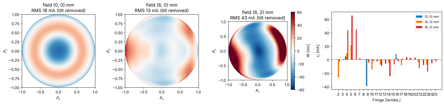
On axis only the rotationally symmetric terms remain (\(Z_4\), \(Z_9\), \(Z_{16}\), \(Z_{25}\): residual spherical aberration balanced with defocus). At the slit edge field curvature (\(Z_4\)), astigmatism (\(Z_5\)), coma (\(Z_7\)) and higher orders appear. 36 Fringe Zernikes describe the wavefront to a few milliwaves.

The fit is checked in the tests against the ray traced PSF: the centroid of the PSF lies at the predicted placement.

2. The scanner slit

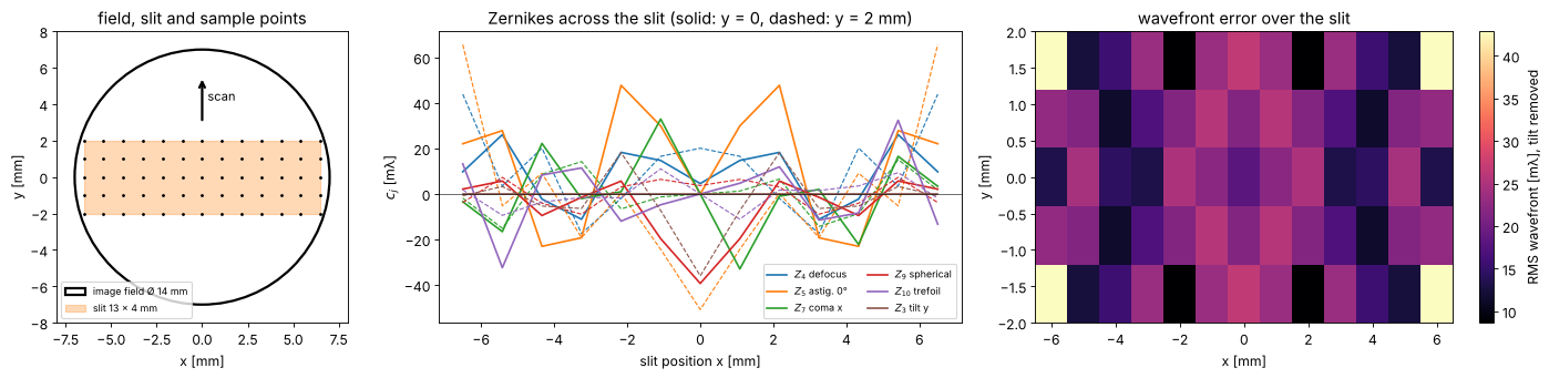
A scanner exposes through a slit, here 13 × 4 mm on the wafer, which just fits into the 14 mm image field of the lens; mask and wafer move along \(y\) (the scan direction) at speeds in the ratio of the magnification. Every point of the wafer is exposed by all scan positions \(y\) of the slit at its slit position \(x\), so the aberrations that matter for imaging vary along \(x\) only, and what varies along \(y\) is averaged.

xs = np.linspace(-SLIT_X, SLIT_X, 13)
ys = np.linspace(-SLIT_Y, SLIT_Y, 5)
grid = [[lens.lens_aberrations(system, (x, y), n_terms=36, N=32) for x in xs] for y in ys]
Z = np.array([[[ab.zernikes[j] for j in range(2, 37)] for ab in row] for row in grid])*1000  # (y, x, j)

fig, axes = plt.subplots(1, 3, figsize=(18, 4.4), gridspec_kw={"width_ratios": [1, 1.6, 1.6]})
ax = axes[0]
ax.add_patch(Circle((0, 0), R_FIELD, fill=False, lw=2, label="image field Ø 14 mm"))
ax.add_patch(Rectangle((-SLIT_X, -SLIT_Y), 2*SLIT_X, 2*SLIT_Y, alpha=0.3, color="C1", label="slit 13 × 4 mm"))
X, Y = np.meshgrid(xs, ys)
ax.plot(X, Y, "k.", ms=3)
ax.annotate("", xy=(0, 5.5), xytext=(0, 3), arrowprops=dict(arrowstyle="->", lw=2))
ax.text(0.3, 4.2, "scan", fontsize=10)
ax.set_aspect("equal"); ax.set_xlim(-8, 8); ax.set_ylim(-8, 8)
ax.set_xlabel("x [mm]"); ax.set_ylabel("y [mm]"); ax.legend(fontsize=8, loc="lower left")
ax.set_title("field, slit and sample points")
labels = {4: "$Z_4$ defocus", 5: "$Z_5$ astig. 0°", 7: "$Z_7$ coma x", 9: "$Z_9$ spherical",
          10: "$Z_{10}$ trefoil", 3: "$Z_3$ tilt y"}
for k, (j, name) in enumerate(labels.items()):
    i = j - 2
    axes[1].plot(xs, Z[len(ys)//2, :, i], "-", color=f"C{k}", label=name)
    axes[1].plot(xs, Z[-1, :, i], "--", color=f"C{k}", lw=1)
axes[1].set_xlabel("slit position x [mm]"); axes[1].set_ylabel("$c_j$ [mλ]")
axes[1].set_title("Zernikes across the slit (solid: y = 0, dashed: y = 2 mm)")
axes[1].legend(fontsize=8, ncol=2); axes[1].axhline(0, color="k", lw=0.5)
W_rms = np.zeros((len(ys), len(xs)))
for r, row in enumerate(grid):
    for c, ab in enumerate(row):
        proj = Projector(NA, WL, n=WATER_ARF, zernikes={j: v for j, v in ab.zernikes.items() if j > 3})
        W_rms[r, c] = 1000*np.std(proj.pupil_phase(PX[inside], PY[inside])/(2*np.pi))
im = axes[2].imshow(W_rms, extent=(xs[0], xs[-1], ys[0], ys[-1]), aspect="auto", cmap="magma")
plt.colorbar(im, ax=axes[2], label="RMS wavefront [mλ], tilt removed")
axes[2].set_xlabel("x [mm]"); axes[2].set_ylabel("y [mm]"); axes[2].set_title("wavefront error over the slit")
fig.tight_layout()

Placement and what the scanner corrects

The chief ray distortion of the design grows towards the corners of the slit (up to about 110 nm, pointing inwards), and the image of a small feature, which lands where the PSF centroid is, follows it closely: coma and the higher order tilts of this well corrected lens add only a few nm. A scanner corrects translation, magnification (along \(x\) in the lens, along \(y\) by the scan speed) and rotation, which linear_correction() fits to the placements of the sample points. Here this removes most of the error: what is left is the nonlinear part, up to about 30 nm in the corners of the slit. In a production lens the residual is a few nm; this design was not optimized for it.

flat = [ab for row in grid for ab in row]
corr = lens.linear_correction(flat)
F = np.array([ab.field for ab in flat])
D_chief = np.array([ab.distortion for ab in flat])
D = np.array([ab.placement for ab in flat])
D_res = D - np.array([corr(*f) for f in F])
T = 1000*np.array([ab.telecentricity for ab in flat])

fig, axes = plt.subplots(2, 2, figsize=(15, 7.5))
axes = axes.ravel()
for ax, d, title in zip(axes, (D_chief, D, D_res),
                        ("chief ray distortion", "placement (PSF centroid)", "after the linear correction")):
    q = ax.quiver(F[:, 0], F[:, 1], d[:, 0], d[:, 1], angles="xy", scale_units="xy", scale=50, width=0.004)
    ax.quiverkey(q, 0.8, 1.06, 50, "50 nm", labelpos="E")
    ax.set_title(f"{title}\nmax {np.max(np.hypot(*d.T)):.0f} nm", fontsize=10)
    ax.set_xlim(-8, 8); ax.set_ylim(-3.5, 3.5); ax.set_aspect("equal"); ax.set_xlabel("x [mm]")
    ax.set_ylabel("y [mm]")
q = axes[3].quiver(F[:, 0], F[:, 1], T[:, 0], T[:, 1], angles="xy", scale_units="xy", scale=20, width=0.004, color="C3")
axes[3].quiverkey(q, 0.8, 1.06, 20, "20 mrad", labelpos="E")
axes[3].set_title(f"telecentricity (chief ray angle)\nmax {np.max(np.hypot(*T.T)):.1f} mrad", fontsize=10)
axes[3].set_xlim(-8, 8); axes[3].set_ylim(-3.5, 3.5); axes[3].set_aspect("equal"); axes[3].set_xlabel("x [mm]")
axes[3].set_ylabel("y [mm]")
fig.tight_layout()
mag_x = corr(1.0, 0.0)[0] - corr(0.0, 0.0)[0]
print(f"fitted magnification error along x: {mag_x:.1f} nm/mm = {mag_x*1e-6:.1e}")
print(f"image shift by telecentricity per 100 nm of defocus at the slit edge: {0.1*np.max(np.hypot(*T.T)):.2f} nm")

fitted magnification error along x: -12.0 nm/mm = -1.2e-05
image shift by telecentricity per 100 nm of defocus at the slit edge: 3.90 nm

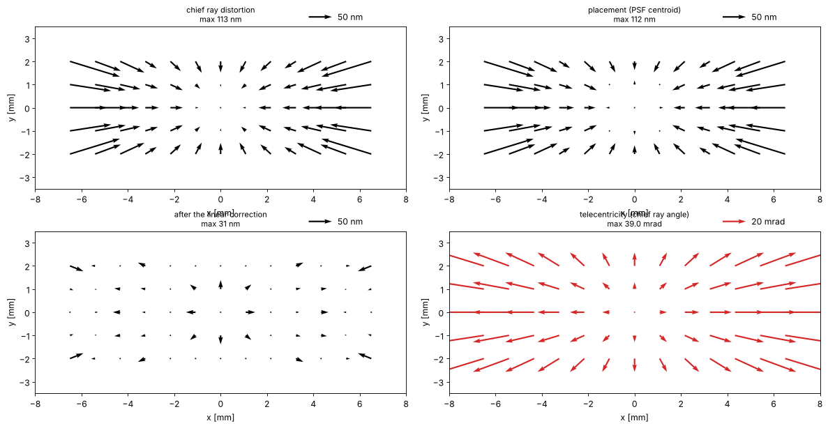
The chief ray in the water is tilted by up to 40 mrad at the edge of the slit, pointing outwards: a defocus of 100 nm moves the image by 4 nm there. This is the one property in which the patent design is far from a scanner lens, whose telecentricity is a few mrad; the focus dependent placement it causes shows up below.

3. CD, placement and best focus across the slit

Three patterns at ArF immersion, binary mask, conventional illumination σ = 0.6 (threshold 0.3, dose to size at the slit centre):

• dense vertical lines, 80 nm lines and spaces (\(k_1 = 0.56\)): the cut goes along \(x\), so \(x\) tilt and \(x\) coma move them,

• the same lines horizontal: the cut goes along \(y\),

• semi-isolated vertical lines, 80 nm at a pitch of 480 nm.

through_slit() computes, at each slit position \(x\), the cuts through focus for all scan positions \(y\) with the Zernikes, placement and telecentricity of the lens there, and averages them: the image a scanned wafer point receives. With only \(y = 0\) it is the static image. Placements are after the linear correction of section 2.

ill = Illumination.conventional(0.6, n_samples=21)
centre = lens.projector_from_system(system, (0.0, 0.0), n=WATER_ARF)
patterns = {"dense V 80/160": MaskLayout.lines_spaces(160.0, 80.0),
            "dense H 80/160": MaskLayout.lines_spaces(160.0, 80.0, orientation="x"),
            "semi-iso V 80/480": MaskLayout.lines_spaces(480.0, 80.0)}
foci = np.linspace(-150, 150, 21)
x_slit = np.linspace(0, SLIT_X, 7)
y_scan = np.linspace(-SLIT_Y, SLIT_Y, 5)
sims, doses, slit = {}, {}, {}
for name, layout in patterns.items():
    sims[name] = LithoSimulation(layout, ThinMask.binary(), ill, centre)
    doses[name] = sims[name].dose_to_size(threshold=0.3)
    for scan, y in (("static", [0.0]), ("scanned", y_scan)):
        slit[name, scan] = lens.through_slit(sims[name], system, x_slit, y=y, dose=doses[name], foci=foci,
                                             correction=corr)

fig, axes = plt.subplots(1, 3, figsize=(18, 4.3))
for k, name in enumerate(patterns):
    for scan, ls in (("static", "--"), ("scanned", "-")):
        r = slit[name, scan]
        lab = f"{name}, {scan}"
        axes[0].plot(r.x, r.cd, ls, color=f"C{k}", marker="o", ms=3, label=lab)
        axes[1].plot(r.x, r.placement, ls, color=f"C{k}", marker="o", ms=3, label=lab)
        axes[2].plot(r.x, r.best_focus, ls, color=f"C{k}", marker="o", ms=3, label=lab)
for ax, yl in zip(axes, ("CD [nm]", "placement [nm] (after linear correction)", "best focus [nm]")):
    ax.set_xlabel("slit position x [mm]"); ax.set_ylabel(yl)
axes[0].legend(fontsize=8)
axes[0].set_title("CD at nominal focus"); axes[1].set_title("placement along the cut"); axes[2].set_title("best focus (largest NILS)")
fig.tight_layout()

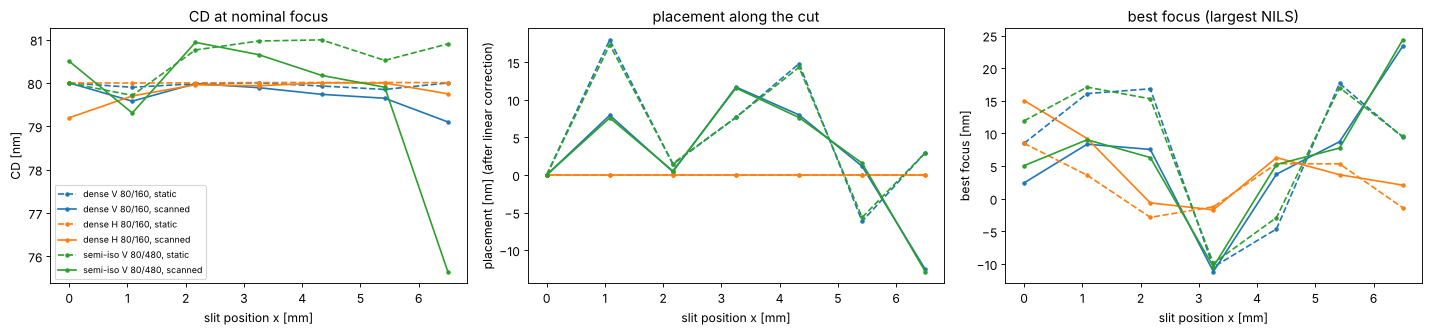
What the curves show:

• CD. The dense lines change by less than 1 nm across the slit, the semi-isolated lines by about 1 nm static and up to 4 nm scanned at the edge. Dense lines at this pitch are imaged by three beams, isolated lines by a continuous spectrum that samples the whole pupil, so they feel more of the wavefront (see section 4).

• Placement. The horizontal lines don’t move: their cut is along \(y\), and the lens is mirror symmetric about \(y = 0\), so the static image has no \(y\) shift, and the scanned image averages \(+y\) and \(-y\). Vertical lines move by the residual distortion (up to 18 nm static, after the linear correction) plus a small pattern dependent coma shift; dense and semi-isolated lines move almost alike here, because the coma of this lens is small.

• Best focus (the focus of the largest NILS) follows the field curvature (\(Z_4\)) and, pattern dependent, spherical aberration and astigmatism: it varies by about 35 nm across the slit, and at the edge vertical and horizontal lines focus up to 20 nm apart (\(Z_5\)).

• Scanning averages the images over \(y\). Where placement or focus vary along \(y\), the averaged image is blurred (image fading), which costs CD and process window; the semi-isolated lines at the slit edge lose 4 nm of CD this way, because their placement and focus change over the 4 mm of the slit along the scan.

Bossung curves at the slit centre and edge

doses_rel = np.linspace(0.85, 1.15, 7)
fig, axes = plt.subplots(1, 3, figsize=(18, 4.3), sharey=True)
for ax, name in zip(axes, patterns):
    for field, ls in (((0.0, 0.0), "-"), ((SLIT_X, 0.0), "--")):
        sim = sims[name].with_(projector=lens.projector_from_system(system, field, n=WATER_ARF))
        fem = sim.fem(foci, doses[name]*doses_rel, 0.3)
        for i, D in enumerate(doses_rel):
            ax.plot(foci, fem[i], ls, color=plt.cm.viridis(i/(len(doses_rel) - 1)),
                    label=f"dose {D:.2f}" if ls == "-" else None)
    ax.set_title(f"{name}\nsolid: slit centre, dashed: x = {SLIT_X:.1f} mm", fontsize=10)
    ax.set_xlabel("focus [nm]"); ax.set_ylim(40, 120)
axes[0].set_ylabel("CD [nm]"); axes[0].legend(fontsize=8, ncol=2)
fig.tight_layout()

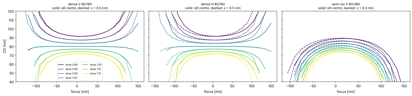
The Bossung curves at the slit centre and edge nearly coincide: the wavefront of the lens is close to the diffraction limit everywhere in the slit. At the edge the curves of the semi-isolated lines shift by some nm in focus and tilt slightly, so the common process window of centre and edge is a little smaller than that of either point.

ideal = Projector(NA, WL, n=WATER_ARF, magnification=8.0)
terms = np.arange(2, 26)
sens = {}
for name in ("dense V 80/160", "semi-iso V 80/480"):
    s = sims[name].with_(projector=ideal)
    sens[name] = lens.zernike_sensitivity(s, terms, delta=0.02, dose=s.dose_to_size(threshold=0.3), foci=foci)

fig, axes = plt.subplots(3, 1, figsize=(15, 10), sharex=True)
panels = [("linear", "placement", "d placement / d$c_j$\n[nm per 10 mλ]"),
          ("linear", "best_focus", "d best focus / d$c_j$\n[nm per 10 mλ]"),
          ("quadratic", "cd", "½ d²CD / d$c_j$² × (10 mλ)²\n[nm]")]
for ax, (order, key, yl) in zip(axes, panels):
    for k, (name, s) in enumerate(sens.items()):
        v = getattr(s, order)[key]*(0.01 if order == "linear" else 0.5*0.01**2)
        ax.bar(terms + (k - 0.5)*0.4, v, 0.4, label=name, color=f"C{2*k}")
    ax.set_xticks(terms); ax.axhline(0, color="k", lw=0.5); ax.set_ylabel(yl)
axes[0].legend(); axes[-1].set_xlabel("Fringe Zernike $j$")
fig.tight_layout()
for name, s in sens.items():
    print(f"{name}: largest |dCD/dc_j| {np.max(np.abs(s.linear['cd'])):.2g} nm per wave")

dense V 80/160: largest |dCD/dc_j| 3.6e-13 nm per wave
semi-iso V 80/480: largest |dCD/dc_j| 3.6e-13 nm per wave

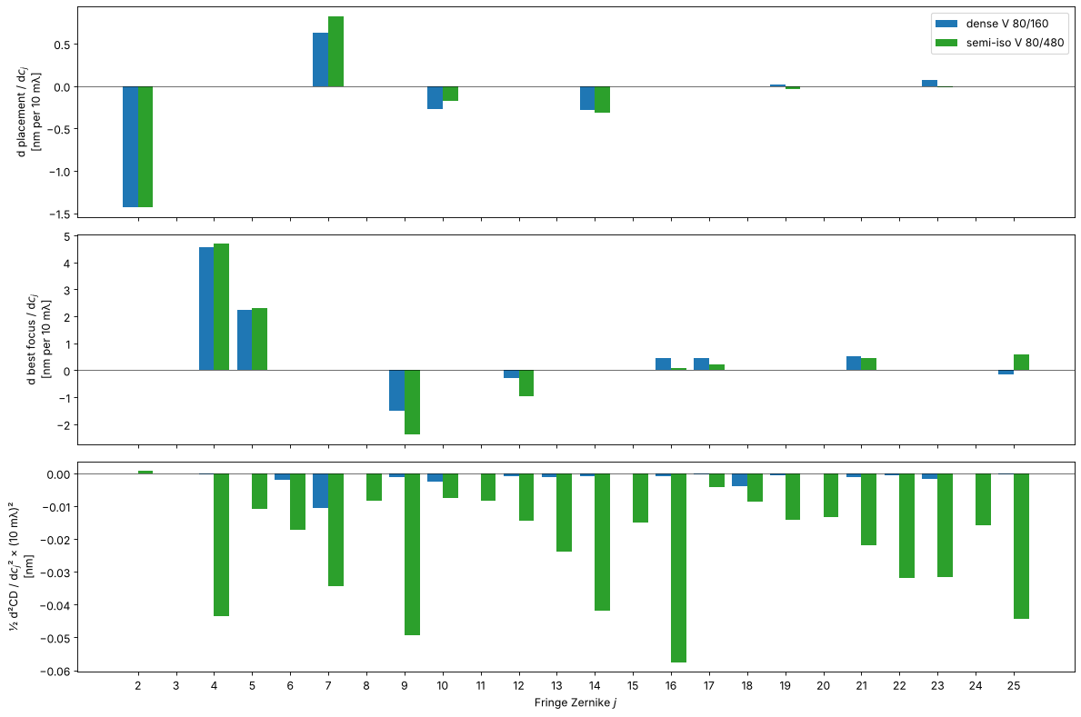
The bars follow from the symmetry of the pattern and the pupil:

• Placement of vertical lines (a cut along \(x\)) responds only to the terms odd in \(x\): tilt \(Z_2\) (exactly \(-\lambda/\mathrm{NA}\) per wave), coma \(Z_7\), trefoil \(Z_{10}\), \(Z_{14}\), \(Z_{19}\), \(Z_{23}\). The even terms leave a symmetric pattern symmetric. How much coma shifts the lines depends on where the diffraction orders pass the pupil, i.e. on the pitch: placement errors are pattern dependent.

• Best focus responds to the even terms: defocus \(Z_4\), spherical aberration \(Z_9\), \(Z_{16}\), and astigmatism \(Z_5\) and \(Z_{12}\) (with opposite signs for horizontal lines). Spherical aberration moves the best focus of dense and isolated lines by different amounts: an iso-dense focus difference.

• CD has no linear sensitivity at all at best focus (printed below): an odd term turns the pattern into its mirror image when its sign changes, and an even term acts near best focus like a small defocus, whose effect on CD is quadratic. The quadratic sensitivities are much larger for the semi-isolated lines, whose spectrum fills the whole pupil. A linear CD sensitivity appears only away from best focus, i.e. through the focus shifts of the second panel.

5. An aberration budget

With the sensitivities, the response to any set of Zernikes is predicted without a new simulation: \(\Delta = \sum_j L_j c_j + \tfrac12 Q_j c_j^2\) (predict()). Applied to the lens Zernikes across the slit, against the full simulation of the static image (Zernikes only, without distortion):

x_fine = np.linspace(0, SLIT_X, 8)
fig, axes = plt.subplots(1, 3, figsize=(18, 4.3))
for k, (name, s) in enumerate(sens.items()):
    sim = sims[name].with_(projector=ideal)
    D = sim.dose_to_size(threshold=0.3)
    sim_r, pred = [], []
    for x in x_fine:
        ab = lens.lens_aberrations(system, (x, 0.0), n_terms=36, N=32)
        r = lens.feature_response(sim.with_(projector=ideal.with_(zernikes=ab.zernikes)), dose=D, foci=foci)
        sim_r.append((r.cd - s.nominal.cd, r.placement - s.nominal.placement, r.best_focus - s.nominal.best_focus))
        p = lens.predict(s, ab.zernikes)
        pred.append((p["cd"], p["placement"], p["best_focus"]))
    sim_r, pred = np.array(sim_r), np.array(pred)
    for i, ax in enumerate(axes):
        ax.plot(x_fine, sim_r[:, i], "o-", color=f"C{2*k}", ms=4, label=f"{name}: simulated")
        ax.plot(x_fine, pred[:, i], "--", color=f"C{2*k}", label=f"{name}: predicted")
for ax, t in zip(axes, ("ΔCD [nm]", "Δ placement [nm]", "Δ best focus [nm]")):
    ax.set_xlabel("slit position x [mm]"); ax.set_ylabel(t); ax.axhline(0, color="k", lw=0.5)
axes[0].legend(fontsize=8)
fig.tight_layout()

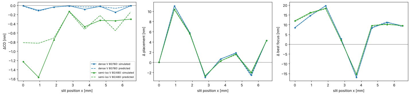
Placement and best focus are predicted well: they are mostly linear in the coefficients. The CD prediction is rougher because CD depends on products of coefficients (defocus times spherical aberration, astigmatism times defocus), which the diagonal model leaves out, and this lens’s aberrations (up to about 65 mλ in single terms) are well beyond the ±20 mλ of the sensitivity steps. For a production lens, with coefficients of a few milliwaves, the linear budget is the standard tool.

Summary

• lens_aberrations() and projector_from_system() hand a ray traced lens to the lithography simulation: Zernikes on the projector’s pupil, distortion, telecentricity and the placement of a small feature.

• Image placement is not chief ray distortion: coma moves the image, and by a pattern dependent amount. Scanners correct the linear part (linear_correction()); the rest is overlay error.

• through_slit() gives CD, placement and best focus across the slit, averaged over the scan; variations along the scan direction fade the image.

• zernike_sensitivity() and predict() give the linear and quadratic sensitivities, their symmetries, and a quick aberration budget.

Exercises: repeat section 3 with an annular or dipole source (the sensitivities of dense lines change completely), stop the lens down (NA=1.2 in lens_aberrations()), run the same steps with the dry KrF lens caldwell_krf_lens() (NA 0.56, telecentric), or shift a lens element with System.with_axial_shift() as in notebook 19 and follow the change of best focus across the slit.

References

• C. Mack, Fundamental Principles of Optical Lithography: The Science of Microfabrication, Wiley (2007).

• A. Erdmann, Optical and EUV Lithography: A Modeling Perspective, SPIE Press (2021).

• J. B. Caldwell, “All-fused-silica 248-nm lithographic projection lens”, Optics & Photonics News 9(11), 40-41 (1998).

• H.-J. Rostalski, A. Dodoc, A. Epple and H. Beierl, “Refractive projection objective for immersion lithography”, US 7,187,503 B2 (2007).

• T. Matsuyama, Y. Ohmura and D. M. Williamson, “The lithographic lens: its history and evolution”, Proc. SPIE 6154, 615403 (2006).