Rigorous mask diffraction (RCWA) and mask 3D effects

So far the mask has been thin: a ThinMask multiplies the illumination by a transmission function, a FilmMask uses the transmission of the absorber film stack for each angle, and an optional BoundaryLayer adds strips at the edges to mimic thick-mask effects. A real absorber is 60–70 nm thick, and at 4× its mask pitch is only one or two wavelengths. The light couples into the absorber sidewalls, and the diffraction orders get amplitudes and phases that the thin models do not have. These are the mask 3D effects: CD offsets, best focus shifts through pitch, and different behaviour for TE and TM.

pyoptics.litho.rcwa solves Maxwell’s equations for lamellar gratings with the rigorous coupled wave analysis (RCWA, Fourier modal method):

• the permittivity of each layer is expanded into Fourier series along the grating, using Li’s factorization rules (the inverse rule for \(E_x\)), which makes TM and metal gratings converge quickly;

• per layer, the modes are the TE and TM modes of the planar problem; any direction of incidence is allowed (conical diffraction);

• layers are stacked with the enhanced transmittance matrix method, which stays stable for thick and absorbing layers.

RigorousMask plugs this into LithoSimulation for 1D layouts. Every source point gets its own orders (Abbe), and hopkins.TCC uses the orders at normal incidence. calibrate_boundary_layer() fits the boundary layer model to the rigorous orders.

Contents:

1. Checks: thin films, energy conservation, convergence.

2. Diffraction orders of a MoSi attenuated PSM: rigorous vs. film mask through pitch.

3. Dependence on the angle of incidence, and the Hopkins approximation.

4. Imaging: CD and best focus through pitch, MoSi and chrome.

5. Calibrating the boundary layer model.

ArF immersion: 193 nm, water, NA 1.35, 4× reduction, mask blank \(n = 1.563\).

import time
import numpy as np
import matplotlib.pyplot as plt

from pyoptics.litho import (Illumination, LithoSimulation, MaskLayout, Projector, RigorousMask,
                            hopkins, lens, rcwa)

plt.rcParams.update({"figure.dpi": 100, "font.size": 11})

wl, n_w, NA, M = 193.0, 1.437, 1.35, 4.0
MOSI, CR, BLANK = 2.343 + 0.586j, 0.84 + 1.65j, 1.563  # as in notebook 32
mosi = RigorousMask([(MOSI, 68.0)], name="MoSi 68 nm (6 % att. PSM)")
chrome = RigorousMask([(CR, 70.0)], name="Cr 70 nm (binary)")
projector = Projector(NA, wl, n=n_w)

1. Checks

rcwa.rcwa() works at mask scale: period, layers (Layer(thickness, background, segments)) and the transverse wave vector of the incident wave in units of \(k_0\). It returns Jones matrices of the reflected and transmitted orders (tangential \(E_x, E_y\)). Three checks:

• an unpatterned stack gives the TE/TM transmissions of thin_films (exact, see the tests);

• a lossless grating conserves energy: the efficiencies of all reflected and transmitted orders sum to 1 for any incidence and polarization;

• convergence with the number of orders: Li’s factorization against the plain Laurent rule for TM light on chrome lines.

grating = [rcwa.Layer(120.0, 1.0, [(0.0, 250.0, 1.5)]), rcwa.Layer(50.0, 1.3, [(100.0, 100.0, 2.0)])]
for k_x, k_y in ((0.0, 0.0), (0.3, 0.0), (-0.5, 0.7)):
    res = rcwa.rcwa(500.0, grating, wl, k_x, k_y, n_in=BLANK, n_out=1.0, n_orders=15)
    sums = [sum(e.sum() for e in res.efficiencies(j)) for j in ([1, 0], [0, 1], [1, 1j])]
    print(f"k = ({k_x:+.1f}, {k_y:+.1f}): R + T = " + ", ".join(f"{s:.15f}" for s in sums))

cr_lines = [rcwa.Layer(70.0, 1.0, [(0.0, 240.0, CR)])]  # 60 nm lines at 120 nm pitch (wafer scale)
orders = np.array([3, 5, 8, 12, 16, 24, 32, 48, 64])
ref = {pol: rcwa.rcwa(480.0, cr_lines, wl, 0.1, 0.0, n_in=BLANK, n_orders=120).t[0, 121, pol, pol]
       for pol in (0, 1)}
fig, ax = plt.subplots(figsize=(7, 4))
for fac, ls in (("li", "-"), ("laurent", "--")):
    for pol, c, name in ((0, "C3", "TM (E across the lines)"), (1, "C0", "TE (E along the lines)")):
        err = [abs(rcwa.rcwa(480.0, cr_lines, wl, 0.1, 0.0, n_in=BLANK, n_orders=k,
                             factorization=fac).t[0, k + 1, pol, pol] - ref[pol]) for k in orders]
        ax.loglog(2*orders + 1, err, ls, color=c, marker="o", ms=3, label=f"{fac}, {name}")
ax.set_xlabel("number of orders"); ax.set_ylabel("error of the first order")
ax.set_title("convergence, Cr lines at 480 nm mask pitch"); ax.legend(fontsize=8); ax.grid(alpha=0.3, which="both")
plt.tight_layout()

k = (+0.0, +0.0): R + T = 0.999999999999997, 1.000000000000001, 0.999999999999999
k = (+0.3, +0.0): R + T = 1.000000000000005, 1.000000000000001, 1.000000000000003
k = (-0.5, +0.7): R + T = 0.999999999999994, 1.000000000000003, 0.999999999999998

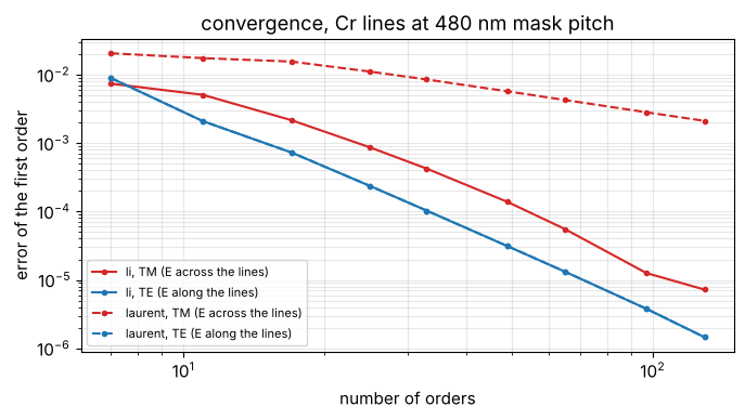
For TE both rules are the same. For TM, Laurent’s rule converges slowly; Li’s inverse rule is about an order of magnitude better. (For TE the two curves lie on top of each other.) RigorousMask keeps roughly twice as many orders as propagate in the blank (at least 21), which gives about \(10^{-3}\) accuracy on the orders that reach the pupil.

2. Diffraction orders through pitch

At normal incidence, lines and spaces with a 1:1 duty cycle on a MoSi attenuated PSM. Thin (film) mask: the orders are the Fourier coefficients of the transmission, independent of polarization, and they scale with pitch. Rigorous: TE and TM orders differ, and their amplitudes and phases change with pitch. The phase of the first order relative to the zeroth acts like a defocus term in the pupil: it shifts best focus differently for each pitch.

pitches = np.linspace(80, 400, 33)
zero = np.zeros(1)
film = mosi.film_mask()
J_abs = film.jones(zero, zero, NA, wl, M)[1][0][0, 0]
a = {"TM": [], "TE": [], "film": []}
for p in pitches:
    layout = MaskLayout.lines_spaces(p, p/2)
    J_o = mosi.order_jones(layout, np.arange(-1, 2), [0], zero, zero, NA, wl, M)[0][:, :, 0]
    a["TM"].append(J_o[0, 0]); a["TE"].append(J_o[1, 1])
    c = layout.region_coefficients(np.arange(-1, 2), [0])
    a["film"].append(c["field"][0] + c["feature"][0]*J_abs)
a = {k: np.array(v) for k, v in a.items()}

fig, axes = plt.subplots(1, 3, figsize=(17, 4.2))
styles = {"TE": ("C0", "-"), "TM": ("C3", "-"), "film": ("k", "--")}
for k, (c, ls) in styles.items():
    axes[0].plot(pitches, np.abs(a[k][:, 1]), ls, color=c, label=k)
    axes[1].plot(pitches, np.abs(a[k][:, 2]), ls, color=c, label=k)
    dphi = np.degrees(np.angle(a[k][:, 2]/a[k][:, 1]))
    axes[2].plot(pitches, dphi, ls, color=c, label=k)
axes[0].set_ylabel("|zeroth order|"); axes[1].set_ylabel("|first order|")
axes[2].set_ylabel("phase(first) − phase(zeroth) [°]")
for ax in axes:
    ax.set_xlabel("pitch (wafer scale) [nm]"); ax.legend(); ax.grid(alpha=0.3)
fig.suptitle("MoSi att. PSM, 1:1 lines and spaces, normal incidence")
plt.tight_layout()

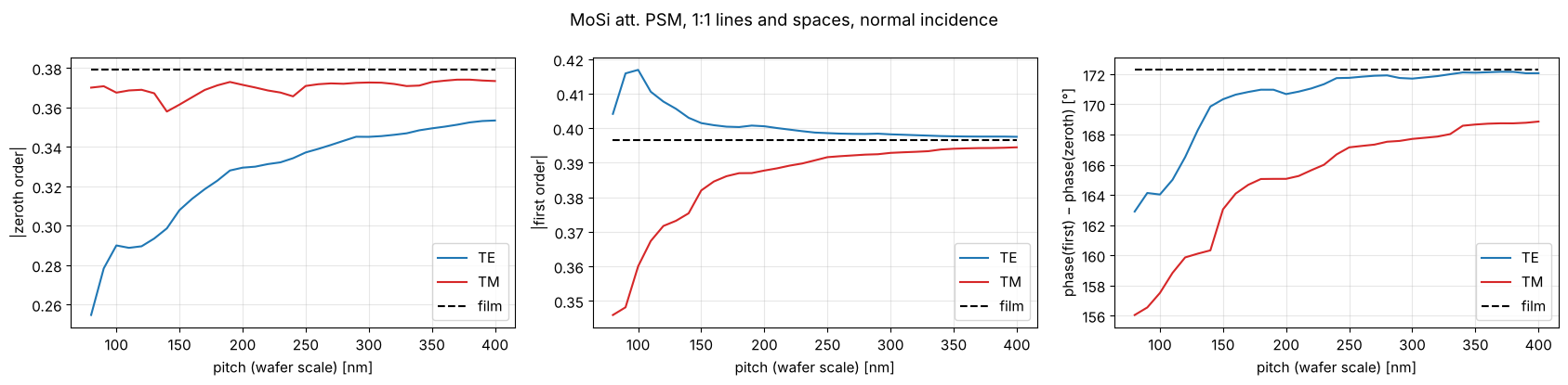
The rigorous orders converge towards the film mask at large pitches. At small pitches the zeroth order (the background) drops in TE, and the first order is stronger in TE and weaker in TM than the film model predicts. The phase difference between the orders is about 172° for the film mask (the MoSi phase at 68 nm; 180° needs a thicker film). In the rigorous mask it drops by up to 16° at small pitches, more in TM. A pupil phase between the orders acts like defocus for that pitch.

3. Angle of incidence and the Hopkins approximation

Each source point illuminates the mask at its own angle: \(\sin\theta = \mathrm{NA}\,s/M\) in air, up to about 0.34. A thin mask diffracts the same orders for every angle (shifted in the pupil). A thick absorber does not: its order amplitudes depend on the angle, by different amounts for each order. The Hopkins TCC assumes normal incidence for all source points; Abbe with RigorousMask recomputes the orders for each one.

layout = MaskLayout.lines_spaces(130.0, 65.0)
s = np.linspace(-1, 1, 41)
J_o = mosi.order_jones(layout, np.arange(-1, 2), [0], s, np.zeros_like(s), NA, wl, M)[:, :, :, 0]
fig, axes = plt.subplots(1, 2, figsize=(13, 4.2))
for i, (m, c) in enumerate(((-1, "C0"), (0, "k"), (1, "C3"))):
    axes[0].plot(s, np.abs(J_o[:, 1, 1, i]), color=c, label=f"order {m:+d}, TE")
    axes[0].plot(s, np.abs(J_o[:, 0, 0, i]), "--", color=c, label=f"order {m:+d}, TM")
axes[0].set_xlabel("source position $s_x$"); axes[0].set_ylabel("|order|")
axes[0].set_title("orders vs. angle of incidence, 130 nm pitch"); axes[0].legend(fontsize=8, ncol=2)

x = np.linspace(-65, 65, 131)
for ill, c in ((Illumination.annular(0.9, 0.6, n_samples=15, polarization="TE"), "C0"),
               (Illumination.dipole(0.95, 0.7, n_samples=15, polarization="y"), "C2")):
    sim = LithoSimulation(layout, mosi, ill, projector)
    I_abbe, I_hop = sim.image(x), hopkins.TCC(sim).image(x)[0]
    axes[1].plot(x, I_abbe, color=c, label=f"{ill.name}: Abbe (rigorous per source point)")
    axes[1].plot(x, I_hop, "--", color=c, label=f"Hopkins, max. difference {np.abs(I_hop - I_abbe).max():.3f}")
axes[1].set_xlabel("x [nm]"); axes[1].set_ylabel("aerial image"); axes[1].legend(fontsize=8)
axes[1].set_title("Abbe vs. Hopkins with a rigorous mask")
for ax in axes:
    ax.grid(alpha=0.3)
plt.tight_layout()

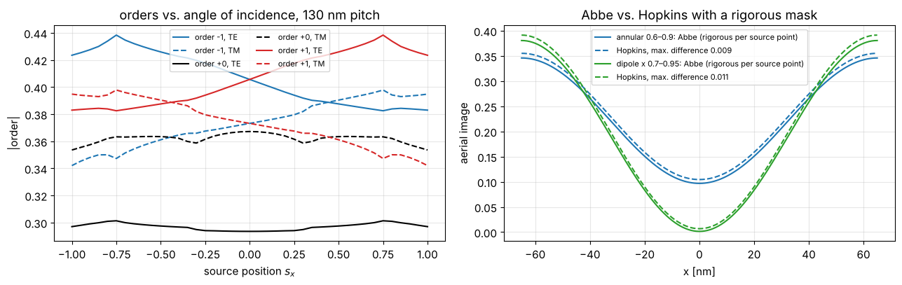
The ±1st orders change by several percent across the source and in opposite directions. Their imbalance across the source acts like a telecentricity error from the mask and tilts the Bossung curves. The Hopkins approximation is good to about a percent of the clear-field intensity here. That is fine for screening; CD-level work needs Abbe.

4. Imaging through pitch

CD at a fixed threshold, and best focus (the vertex of NILS through focus, as in notebook 33), for the rigorous masks and their film approximations. TE-polarized annular illumination.

ill = Illumination.annular(0.9, 0.6, n_samples=15, polarization="TE")
pitches_img = np.array([100, 115, 130, 150, 180, 220, 260, 320, 400])
foci = np.linspace(-80, 80, 9)
results = {}
t0 = time.time()
for rig in (mosi, chrome):
    for stack, kind in ((rig, "rigorous"), (rig.film_mask(), "film")):
        r = [lens.feature_response(LithoSimulation(MaskLayout.lines_spaces(p, p/2), stack, ill, projector),
                                   threshold=0.25, foci=foci) for p in pitches_img]
        results[rig.name, kind] = (np.array([x.cd for x in r]), np.array([x.best_focus for x in r]))
print(f"{time.time() - t0:.1f} s")

fig, axes = plt.subplots(1, 2, figsize=(13, 4.2))
for rig, c in ((mosi, "C0"), (chrome, "C3")):
    for kind, ls in (("rigorous", "-"), ("film", "--")):
        cd, bf = results[rig.name, kind]
        axes[0].plot(pitches_img, cd - pitches_img/2, ls, marker="o", ms=3, color=c, label=f"{rig.name}, {kind}")
        axes[1].plot(pitches_img, bf, ls, marker="o", ms=3, color=c, label=f"{rig.name}, {kind}")
axes[0].set_ylabel("CD − mask CD [nm] (threshold 0.25)"); axes[0].set_title("CD through pitch")
axes[1].set_ylabel("best focus [nm]"); axes[1].set_title("best focus through pitch")
for ax in axes:
    ax.set_xlabel("pitch [nm]"); ax.legend(fontsize=8); ax.grid(alpha=0.3)
plt.tight_layout()

7.6 s

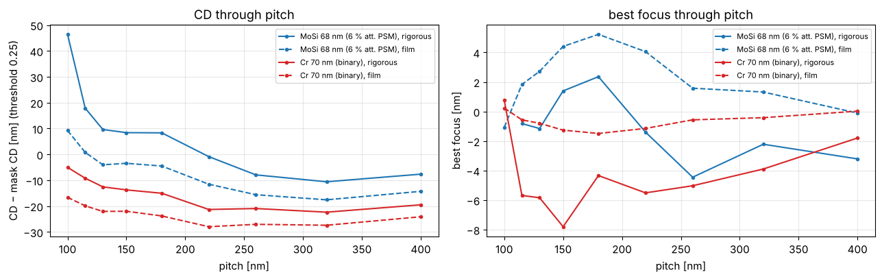
The rigorous lines print wider than the film model predicts: by 5 to 10 nm for chrome, and by 7 nm at large pitches up to 37 nm at 100 nm pitch for MoSi. The thick absorber edges block more light than a thin absorber of the same width. This is a mask bias that OPC has to correct, and it depends on the material. Best focus through pitch also differs between the two models, by several nanometres (up to 8 nm for chrome). These are the effects that thin mask models must be calibrated for.

5. Calibrating the boundary layer model

The boundary layer model puts strips of width \(w\) with transmissions \(t_\mathrm{TE}\) and \(t_\mathrm{TM}\) on every edge. For a given \(w\) the orders are linear in the two transmissions, so calibrate_boundary_layer() fits them by least squares to the rigorous orders of a set of layouts at normal incidence and scans \(w\). The calibrated FilmMask with BoundaryLayer is as fast as the thin models.

cal_layouts = [MaskLayout.lines_spaces(p, p/2) for p in (100, 130, 180, 260, 400)]
cals = {rig.name: rcwa.calibrate_boundary_layer(rig, cal_layouts, NA, wl, M) for rig in (mosi, chrome)}
fig, axes = plt.subplots(1, 2, figsize=(13, 4.2))
for (name, cal), c in zip(cals.items(), ("C0", "C3")):
    bl = cal.boundary_layer
    print(f"{name}: w = {bl.width:.1f} nm, t_TE = {bl.t_TE:.3f}, t_TM = {bl.t_TM:.3f}, "
          f"residual of the orders {100*cal.residual.min():.1f} % "
          f"(film mask alone: {100*cal.residual_base:.1f} %)")
    axes[0].plot(cal.widths, 100*cal.residual, color=c, label=name)

for rig, c in ((mosi, "C0"), (chrome, "C3")):
    cd_rig = results[rig.name, "rigorous"][0]
    cd_film = results[rig.name, "film"][0]
    cd_bl = np.array([LithoSimulation(MaskLayout.lines_spaces(p, p/2), cals[rig.name].stack, ill, projector)
                      .cd(0.25) for p in pitches_img])
    axes[1].plot(pitches_img, cd_film - cd_rig, "--", marker="o", ms=3, color=c, label=f"{rig.name}: film")
    axes[1].plot(pitches_img, cd_bl - cd_rig, "-", marker="o", ms=3, color=c, label=f"{rig.name}: film + boundary layer")
axes[0].set_xlabel("boundary layer width w [nm]"); axes[0].set_ylabel("rms residual of the orders [%]")
axes[0].set_title("fit residual vs. width"); axes[0].legend()
axes[1].axhline(0, color="gray", lw=0.8)
axes[1].set_xlabel("pitch [nm]"); axes[1].set_ylabel("CD error vs. rigorous [nm]")
axes[1].set_title("thin models against RCWA (TE annular)"); axes[1].legend(fontsize=8)
for ax in axes:
    ax.grid(alpha=0.3)
plt.tight_layout()

MoSi 68 nm (6 % att. PSM): w = 7.5 nm, t_TE = -0.320-0.041j, t_TM = 0.205+0.577j, residual of the orders 6.5 % (film mask alone: 13.3 %)
Cr 70 nm (binary): w = 9.5 nm, t_TE = 0.283-0.443j, t_TM = 0.227+0.249j, residual of the orders 7.7 % (film mask alone: 12.9 %)

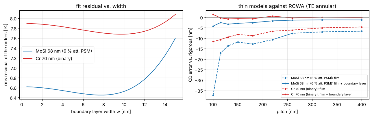
The calibrated boundary layer brings the CD through pitch to within 1 to 4 nm of the rigorous result, against 5 to 37 nm for the film mask alone. It needs only one width and two complex transmissions per material. The fit depends little on the width: narrow strips with stronger transmissions do about as well as wide ones. What remains comes from what a boundary layer cannot represent: the angle dependence of section 3 (the calibration is at normal incidence) and the coupling between neighbouring edges at the smallest pitches.

Summary

• rcwa.rcwa(): RCWA of lamellar gratings with Li’s factorization, conical incidence and stable stacking; exact for unpatterned stacks and energy-conserving for lossless gratings.

• RigorousMask: a mask stack for 1D layouts in LithoSimulation (orders per source point) and hopkins.TCC (orders at normal incidence).

• Mask 3D effects: polarization-dependent order amplitudes, phase errors between the orders, angle dependence, CD offsets of tens of nanometres and best focus shifts through pitch that thin masks miss.

• calibrate_boundary_layer() turns RCWA into a fast, calibrated thin mask model.

• Limitations: 1D layouts only (no contact holes), and the Hopkins approximation for the TCC.

References

• M. G. Moharam and T. K. Gaylord, “Rigorous coupled-wave analysis of planar-grating diffraction”, J. Opt. Soc. Am. 71, 811-818 (1981).

• M. G. Moharam, D. A. Pommet, E. B. Grann and T. K. Gaylord, “Stable implementation of the rigorous coupled-wave analysis for surface-relief gratings: enhanced transmittance matrix approach”, J. Opt. Soc. Am. A 12, 1077-1086 (1995).

• P. Lalanne and G. M. Morris, “Highly improved convergence of the coupled-wave method for TM polarization”, J. Opt. Soc. Am. A 13, 779-784 (1996).

• L. Li, “Use of Fourier series in the analysis of discontinuous periodic structures”, J. Opt. Soc. Am. A 13, 1870-1876 (1996).

• J. Tirapu-Azpiroz, P. Burchard and E. Yablonovitch, “Boundary layer model to account for thick mask effects in photolithography”, Proc. SPIE 5040, 1611 (2003).

• A. Erdmann, Optical and EUV Lithography: A Modeling Perspective, SPIE Press (2021).