Propagation in inhomogeneous media: the wave propagation method (WPM)

The FFT propagators from notebook 01 assume a homogeneous medium. The wave propagation method by Brenner and Singer (pyoptics.wpm) extends the idea to media with a spatially varying refractive index \(n(x, y, z)\): the field is propagated in thin slices \(\Delta z\). In each slice it is decomposed into plane waves, and every plane wave is propagated at every location with the local \(k_z(x, y) = \sqrt{n(x, y)^2 k_0^2 - k_x^2 - k_y^2}\):

\[U(x, y, z + \Delta z) = \sum_{k_x, k_y} \tilde U(k_x, k_y; z)\, e^{i(k_x x + k_y y)}\, e^{i k_z(x, y)\,\Delta z}.\]

Summed directly, this costs \(O(N_x^2 N_y^2)\) per step (method="direct"). If the slice consists of a few materials only, the same sum can be rearranged: for each distinct index \(n_q\), the whole spectrum is propagated with the homogeneous transfer function of \(n_q\) by FFT, and each pixel takes the result of its own material (method="levels", the “fast WPM”). Both give the same result to rounding errors; the default method="auto" picks the cheaper one. The index is sampled in the middle of each slice by default (n_sampling).

For problems that are invariant in \(y\) (\(xz\) cuts through waveguides, cylindrical lenses, …) the field can be one-dimensional: pass y=None. wpm_propagate_z() steps through a list of \(z\) positions and returns the field at all of them.

Sampling: the plane wave decomposition contains all propagating waves of the densest medium only if \(\Delta x \leq \lambda / (2 n_\mathrm{max})\) (max_sampling_distance()).

Note: wpm.pyx is a Cython extension and is compiled when pyoptics is installed.

import time

import numpy as np
import matplotlib.pyplot as plt
from matplotlib import colormaps
from matplotlib.colors import ListedColormap

from pyoptics.wpm import wpm_propagate_z, max_sampling_distance
from pyoptics import propagators as prop
from pyoptics.utils import grid1d

plt.rcParams.update({"figure.dpi": 100, "image.origin": "lower", "font.size": 11, "figure.facecolor": "white"})

# intensities on light backgrounds: reversed magma, faded to white at zero
_t = np.linspace(0, 1, 256)[:, None]
light = ListedColormap(1 - (1 - colormaps["magma_r"](_t[:, 0])[:, :3])*np.clip(_t/0.15, 0, 1), name="light")

wl = 1.0                 # wavelength [µm]
k0 = 2*np.pi/wl

def run_wpm(n_xz, u0, x, z_vals, **kwargs):
    """Propagate u0(x) through n(x, z) (y-invariant) and return the field at all z_vals.
    n_xz(X, z) returns the index on the grid X for the slice at z."""
    return wpm_propagate_z(lambda X, Y, z: n_xz(X, z), u0, x, None, z_vals, wl, **kwargs)

def plot_xz(ax, U, x, z_vals, n_map=None, title="", xlim=None, gamma=1.0):
    I = np.abs(U)**2
    ax.imshow(((I/I.max())**gamma).T, extent=(z_vals[0], z_vals[-1], x[0], x[-1]), aspect="auto",
              cmap=light, interpolation="bilinear")
    if n_map is not None:
        ax.contour(z_vals, x, n_map.T, levels=np.unique(np.round(n_map, 4))[:-1] + 1e-4,
                   colors="0.3", linewidths=0.6, alpha=0.7)
    ax.set_xlabel("$z$ [µm]"); ax.set_ylabel("$x$ [µm]"); ax.set_title(title)
    if xlim:
        ax.set_ylim(*xlim)

1. Test: homogeneous medium

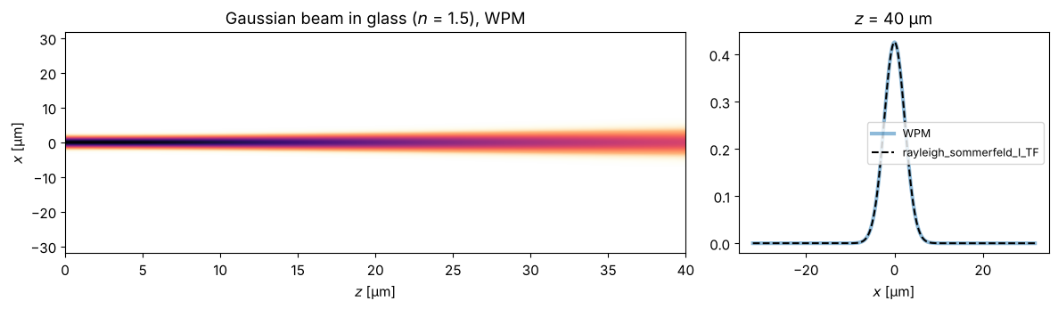
In a homogeneous medium, the WPM must give exactly the result of the Rayleigh-Sommerfeld propagator (transfer function with \(n\)). The comparison uses the 2D propagator on a grid with two \(y\) rows (a \(y\)-invariant field). We also time both implementations of the WPM sum: with only one index value, "levels" needs a single FFT pair per step.

L, N = 64.0, 256
x = grid1d(-L/2, L/2, N)
print(f"dx = {x[1] - x[0]:.3f} µm, max. dx for n = 1.5: {max_sampling_distance(wl, 1.5):.3f} µm")
u0 = np.exp(-x**2/2.0**2)
z_vals = np.linspace(0, 40, 81)
n_glass = lambda X, z: 1.5*np.ones_like(X)

for method in ("direct", "levels"):
    t0 = time.time()
    U_wpm = run_wpm(n_glass, u0, x, z_vals, method=method)
    print(f"80 WPM steps, method='{method}': {time.time() - t0:.3f} s")
y2 = grid1d(-1, 1, 2)    # two y rows: problem invariant in y
U_rs, _, _ = prop.rayleigh_sommerfeld_I_TF(np.tile(u0, (2, 1)).astype(complex), x, y2, z_vals[-1], wl, n=1.5)
print(f"max. deviation from RS: {np.abs(U_wpm[-1] - U_rs[0]).max():.1e}")

fig, axes = plt.subplots(1, 2, figsize=(12, 3.6), gridspec_kw={"width_ratios": [2, 1]})
plot_xz(axes[0], U_wpm, x, z_vals, title="Gaussian beam in glass ($n$ = 1.5), WPM")
axes[1].plot(x, np.abs(U_wpm[-1])**2, lw=3, alpha=0.5, label="WPM")
axes[1].plot(x, np.abs(U_rs[0])**2, "k--", label="rayleigh_sommerfeld_I_TF")
axes[1].set_xlabel("$x$ [µm]"); axes[1].set_title(f"$z$ = {z_vals[-1]:.0f} µm"); axes[1].legend(fontsize=9)
fig.tight_layout()

dx = 0.250 µm, max. dx for n = 1.5: 0.333 µm

80 WPM steps, method='direct': 0.329 s
80 WPM steps, method='levels': 0.016 s
max. deviation from RS: 7.6e-15

2. Gradient-index (GRIN) lens

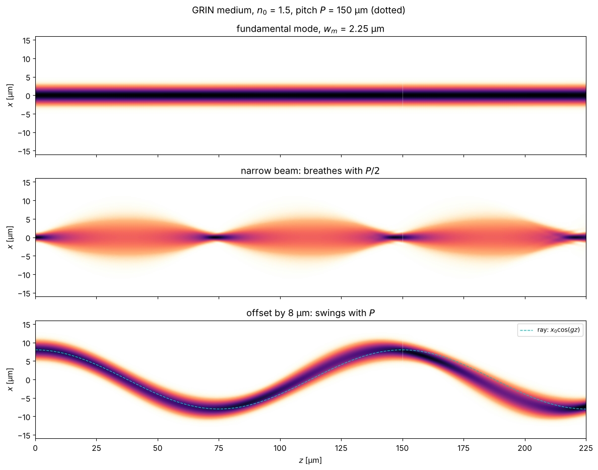
A parabolic index profile \(n(x) = n_0\,(1 - g^2 x^2/2)\) acts like a continuous sequence of weak lenses. Rays oscillate sinusoidally about the axis, \(x(z) = x_0\cos(gz)\), with the pitch length \(P = 2\pi/g\). A Gaussian beam with the radius \(w_m = \sqrt{2/(k_0 n_0 g)}\) is the fundamental mode of the profile and propagates unchanged. A narrower beam “breathes” with the period \(P/2\), an offset one swings like the ray of geometrical optics. (Shown is \(I^{0.6}\), so that the weak parts stay visible.) The profile is continuous, so almost every pixel has its own index, and method="auto" uses the direct sum here.

The offset beam swings somewhat more slowly than the paraxial ray \(x_0\cos(gz)\): at 8 µm displacement it is no longer strictly paraxial.

n0, P = 1.5, 150.0
g = 2*np.pi/P
# clip the profile at n = 1.3 near the edge, otherwise the index would drop below 1 at the window edge:
n_grin = lambda X, z: np.maximum(n0*(1 - g**2*X**2/2), 1.3)
w_m = np.sqrt(2/(k0*n0*g))
z_vals = np.linspace(0, 1.5*P, 451)

beams = ((np.exp(-x**2/w_m**2), f"fundamental mode, $w_m$ = {w_m:.2f} µm"),
         (np.exp(-x**2/(w_m/2.5)**2), "narrow beam: breathes with $P/2$"),
         (np.exp(-(x - 8)**2/w_m**2), "offset by 8 µm: swings with $P$"))
fig, axes = plt.subplots(3, 1, figsize=(12, 9.5), sharex=True)
for ax, (u, title) in zip(axes, beams):
    U = run_wpm(n_grin, u, x, z_vals)
    plot_xz(ax, U, x, z_vals, title=title, xlim=(-16, 16), gamma=0.6)
    for m in range(1, 2):
        ax.axvline(m*P, color="w", lw=0.6, ls=":")
axes[2].plot(z_vals, 8*np.cos(g*z_vals), "c--", lw=1, label="ray: $x_0\\cos(gz)$")
axes[2].legend(loc="upper right", fontsize=9)
for ax in axes[:2]:
    ax.set_xlabel("")
fig.suptitle(f"GRIN medium, $n_0$ = {n0}, pitch $P$ = {P:.0f} µm (dotted)")
fig.tight_layout()

3. Step-index waveguide

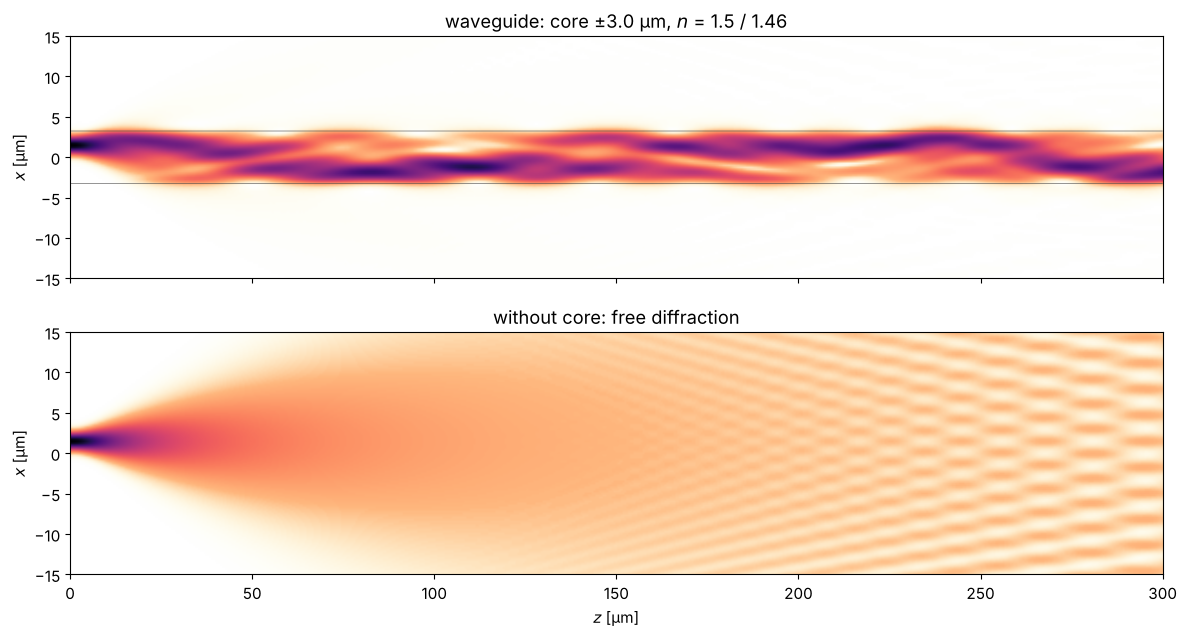
A core with a higher index traps light by total internal reflection. In the wave picture: the core supports guided modes whose field decays evanescently in the cladding. A Gaussian beam that does not exactly match the fundamental mode excites several modes, which travel with different propagation constants and beat against each other. Without a core (bottom) the beam simply diffracts apart. With two index values, method="auto" uses the fast "levels" sum.

core, n_core, n_clad = 3.0, 1.50, 1.46
n_wg = lambda X, z: np.where(np.abs(X) <= core, n_core, n_clad)
NA_wg = np.sqrt(n_core**2 - n_clad**2)
V = k0*core*NA_wg
print(f"NA = {NA_wg:.3f}, V parameter (half core width) = {V:.2f} -> about {int(2*V/np.pi) + 1} guided modes")
z_vals = np.linspace(0, 300, 601)
u_in = np.exp(-(x - 1.5)**2/1.2**2)   # narrow and slightly offset: excites several modes

U_wg = run_wpm(n_wg, u_in, x, z_vals)
U_free = run_wpm(lambda X, z: n_clad*np.ones_like(X), u_in, x, z_vals)
n_map = np.array([n_wg(x, z) for z in z_vals])

fig, axes = plt.subplots(2, 1, figsize=(12, 6.5), sharex=True)
plot_xz(axes[0], U_wg, x, z_vals, n_map=n_map, title=f"waveguide: core ±{core} µm, $n$ = {n_core} / {n_clad}",
        xlim=(-15, 15), gamma=0.6)
plot_xz(axes[1], U_free, x, z_vals, title="without core: free diffraction", xlim=(-15, 15), gamma=0.6)
axes[0].set_xlabel("")
fig.tight_layout()

NA = 0.344, V parameter (half core width) = 6.49 -> about 5 guided modes

P_core = [np.sum(np.abs(U[np.abs(x) <= core])**2)/np.sum(np.abs(U)**2) for U in U_wg]
P_free = [np.sum(np.abs(U[np.abs(x) <= core])**2)/np.sum(np.abs(U)**2) for U in U_free]
fig, ax = plt.subplots(figsize=(8, 3.2))
ax.plot(z_vals, P_core, label="with core")
ax.plot(z_vals, P_free, label="without core")
ax.set_xlabel("$z$ [µm]"); ax.set_ylabel("power fraction in $|x| \\leq$ " + f"{core} µm")
ax.set_ylim(0, 1.05); ax.legend()
fig.tight_layout()

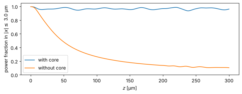
Part of the power is lost at the beginning: it belongs to radiation modes that are not guided and radiate sideways. (At the window edge, this light re-enters on the other side because of the periodic boundary conditions of the plane-wave decomposition. For longer distances, an absorbing index \(n + i\kappa\) near the window edges takes it out.)

4. A thick cylindrical lens

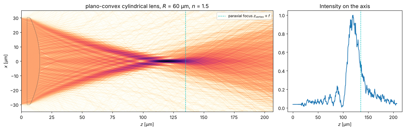
Finally, a case the WPM is made for: a large index step at a curved surface. A plano-convex cylindrical glass lens (\(n = 1.5\)) with radius of curvature \(R\) has the focal length \(f = R/(n-1)\), measured from the principal plane, which for a plano-convex lens lies at the vertex of the curved surface. With \(\pm 30\) µm at \(R = 60\) µm, however, the aperture is anything but paraxial. The WPM shows the focus including spherical aberration: marginal rays cross the axis too early, the intensity maximum lies well before the paraxial focus, and a caustic forms in front of the focus.

L4, N4 = 96.0, 512
x4 = grid1d(-L4/2, L4/2, N4)
R_lens, n_lens, z_front, half_ap = 60.0, 1.5, 5.0, 30.0
sag = R_lens - np.sqrt(np.maximum(R_lens**2 - x4**2, 0))
t_center = R_lens - np.sqrt(R_lens**2 - half_ap**2) + 2.0   # centre thickness
z_vertex = z_front + t_center   # vertex of the curved back surface

def n_lens_func(X, z):
    # flat front surface at z_front, curved back surface: z <= z_vertex - sag(x)
    s = R_lens - np.sqrt(np.maximum(R_lens**2 - X**2, 0))
    inside = (z >= z_front) & (z <= z_vertex - s) & (np.abs(X) <= half_ap)
    return np.where(inside, n_lens, 1.0)

f = R_lens/(n_lens - 1)
z_vals = np.linspace(0, z_vertex + 1.6*f, 700)
u_plane = np.where(np.abs(x4) <= half_ap, 1.0, 0.0)*np.exp(-(x4/40)**8)  # plane wave with soft edges
t0 = time.time()
U_lens = run_wpm(n_lens_func, u_plane, x4, z_vals)
print(f"{len(z_vals) - 1} WPM steps with N = {N4}: {time.time() - t0:.1f} s")
n_map = np.array([n_lens_func(x4, z) for z in z_vals])

fig, axes = plt.subplots(1, 2, figsize=(14, 4.6), gridspec_kw={"width_ratios": [2.2, 1]})
plot_xz(axes[0], U_lens, x4, z_vals, n_map=n_map, title=f"plano-convex cylindrical lens, $R$ = {R_lens:.0f} µm, $n$ = {n_lens}",
        xlim=(-35, 35), gamma=0.5)
axes[0].axvline(z_vertex + f, color="c", ls="--", lw=1, label="paraxial focus $z_\\mathrm{vertex} + f$")
axes[0].legend(loc="upper right", fontsize=9)
I_axis = np.abs(U_lens[:, N4//2])**2
axes[1].plot(z_vals, I_axis/I_axis.max())
axes[1].axvline(z_vertex + f, color="c", ls="--", lw=1)
axes[1].set_xlabel("$z$ [µm]"); axes[1].set_title("Intensity on the axis")
fig.tight_layout()
z_peak = z_vals[np.argmax(I_axis)]
print(f"paraxial focus at z = {z_vertex + f:.1f} µm, intensity maximum at z = {z_peak:.1f} µm")

699 WPM steps with N = 512: 0.2 s
paraxial focus at z = 135.0 µm, intensity maximum at z = 119.7 µm

5. Ball lens and circular cylinder: comparison with the exact solution

A glass sphere is the simplest thick lens, and a popular one: ball lenses couple light into fibres and collimate the light of laser diodes. In paraxial optics, a ball of diameter \(D\) and index \(n\) has the effective focal length

\[f = \frac{n D}{4 (n - 1)},\]

measured from the centre (both principal planes lie there), and the back focal length \(f - D/2\). For \(n = 1.5\) and \(D = 20\) µm: \(f = 15\) µm, 5 µm behind the ball. The aperture is as large as it gets: at the rim, the light hits the surface at grazing incidence, so the spherical aberration is strong and the WPM is tested at steep interfaces.

In contrast to the plano-convex lens above, a sphere and a circular cylinder have exact solutions as series of multipoles: Lorenz-Mie theory for the sphere and its two-dimensional counterpart for the cylinder. For a cylinder lit with \(E\) parallel to its axis (TE), \(E_y\) obeys exactly the scalar Helmholtz equation \(\nabla^2 u + k_0^2 n^2 u = 0\), which the WPM approximates, with \(u\) and \(\partial u/\partial r\) continuous at the surface. The series is a true solution of Maxwell’s equations and the ideal reference for the WPM with 1D fields. For a sphere, the electric field depends on the polarization; the WPM’s scalar wave equation has its own exact solution, the same kind of series with spherical Bessel functions (the “acoustic” sphere). Both are in pyoptics.analytical:

• cylinder_field(): \(u = \sum_m i^m B_m \left[J_m(kr) + a_m H_m(kr)\right] e^{im\varphi}\) outside, \(\sum_m i^m B_m c_m J_m(nkr)\, e^{im\varphi}\) inside,

• sphere_field(): \(u = \sum_l i^l (2l+1) B_l \left[j_l(kr) + a_l h_l(kr)\right] P_l(\cos\theta)\) outside, \(\sum_l i^l (2l+1) B_l c_l j_l(nkr)\, P_l(\cos\theta)\) inside.

The coefficients \(B_m\), \(B_l\) describe the incident field. For a plane wave they are 1. For a beam, they follow from its angular spectrum, so that the exact solution and the WPM can start from exactly the same beam (the simplest case of “generalized Lorenz-Mie theory”). We use a flat top \(e^{-(r/w)^6}\) with \(w = 15\) µm in the plane through the centre; the WPM starts 3 µm in front of the lens with that beam propagated back to there.

The exact solution contains everything the WPM leaves out: reflection at both surfaces (amplitude transmission \(t_1 = 2/(1+n)\) and \(t_2 = 2n/(1+n)\) at normal incidence, \((t_1 t_2)^2 = 0.92\) in intensity, and much less at grazing incidence), multiply reflected light inside the ball, and resonances.

from scipy.special import j0
from pyoptics.analytical import cylinder_field, sphere_field
from pyoptics.wpm import wpm_propagate

n_ball, a_ball = 1.5, 10.0          # index and radius [µm]
efl = n_ball*2*a_ball/(4*(n_ball - 1))
print(f"D = {2*a_ball:.0f} µm, n = {n_ball}: EFL = {efl:.1f} µm from the centre, BFL = {efl - a_ball:.1f} µm")

def flat_top(r, w=15.0):
    # illumination in the plane z = 0 through the centre: flat top with soft edges
    return np.exp(-(r/w)**6)

def back_propagate(u, kx, ky, z):
    # homogeneous propagation (air) of a field u(x, y) or u(x) over z by its angular spectrum
    KZ = np.sqrt((k0**2 - kx**2 - ky**2).astype(complex))
    axes = tuple(range(-u.ndim, 0))
    return np.fft.ifftn(np.fft.fftn(u, axes=axes)*np.exp(1j*KZ*z)*(KZ.imag == 0), axes=axes)

# --- circular cylinder (axis along y), TE: WPM with 1D fields -------------------------
Lb, Nb = 96.0, 512
xb = grid1d(-Lb/2, Lb/2, Nb)        # xb[Nb//2] = 0
kxb = 2*np.pi*np.fft.fftfreq(Nb, xb[1] - xb[0])
z0b = -a_ball - 3.0                 # start of the WPM, 3 µm in front of the lens
u0b = back_propagate(np.fft.ifftshift(flat_top(xb)), kxb, 0*kxb, z0b)
u0b = np.fft.fftshift(u0b)
n_cyl = lambda X, z: np.where(X**2 + z**2 < a_ball**2, n_ball, 1.0)
z_b = np.arange(z0b, 40.0 + 1e-9, 0.1)
t0 = time.time()
U_cyl = run_wpm(n_cyl, u0b, xb, z_b)
print(f"cylinder: {len(z_b) - 1} WPM steps: {time.time() - t0:.1f} s")

# exact solution for the same incident field: its plane waves, phases referred to the centre
A_b = np.fft.fft(np.fft.ifftshift(flat_top(xb)))/Nb
prop_b = np.abs(kxb) < k0
z_e, x_e = z_b[::4], xb[np.abs(xb) <= 25]
t0 = time.time()
U_cyl_exact = cylinder_field(x_e[None, :], z_e[:, None], a_ball, n_ball, wl, k_x=kxb[prop_b], amplitudes=A_b[prop_b])
print(f"cylinder: exact solution on {U_cyl_exact.size} points: {time.time() - t0:.1f} s")

fig = plt.figure(figsize=(13, 7.2))
gs = fig.add_gridspec(2, 3, width_ratios=[2.2, 1, 1])
ax_w, ax_e = fig.add_subplot(gs[0, 0]), fig.add_subplot(gs[1, 0])
n_map_b = np.array([n_cyl(x_e, z) for z in z_e])
on_e = np.abs(x_e) <= 25
plot_xz(ax_w, U_cyl[::4][:, np.abs(xb) <= 25], x_e, z_e, n_map=n_map_b, title="WPM", gamma=0.5)
plot_xz(ax_e, U_cyl_exact, x_e, z_e, n_map=n_map_b, title="exact (cylinder series)", gamma=0.5)
for ax in (ax_w, ax_e):
    ax.axvline(efl, color="C0", ls="--", lw=1)
ax_w.text(efl + 0.5, 21, "paraxial focus", color="C0", fontsize=9)

ax_ax = fig.add_subplot(gs[0, 1:])
ax_ax.plot(z_b, np.abs(U_cyl[:, Nb//2])**2, lw=3, alpha=0.5, label="WPM")
ax_ax.plot(z_e, np.abs(U_cyl_exact[:, len(x_e)//2])**2, "k", lw=0.9, label="exact")
ax_ax.axvspan(-a_ball, a_ball, color="0.92", zorder=-1)
ax_ax.axvline(efl, color="C0", ls="--", lw=1)
ax_ax.set_xlabel("$z$ [µm]"); ax_ax.set_ylabel("$|u|^2$"); ax_ax.set_title("on the axis")
ax_ax.legend(fontsize=9)

k_f = np.argmax(np.abs(U_cyl_exact[:, len(x_e)//2]))
k_fw = np.argmin(np.abs(z_b - z_e[k_f]))
for ax, xl in ((fig.add_subplot(gs[1, 1]), 25), (fig.add_subplot(gs[1, 2]), 4)):
    ax.plot(xb, np.abs(U_cyl[k_fw])**2, lw=3, alpha=0.5, label="WPM")
    ax.plot(x_e, np.abs(U_cyl_exact[k_f])**2, "k", lw=0.9, label="exact")
    ax.set_xlim(-xl, xl); ax.set_xlabel("$x$ [µm]")
    ax.set_title(f"$z$ = {z_e[k_f]:.1f} µm (best focus)" if xl > 10 else "zoom")
fig.suptitle(f"circular cylinder, $D$ = {2*a_ball:.0f} µm, $n$ = {n_ball}, TE", y=1.0)
fig.tight_layout()
I_w, I_e = np.abs(U_cyl[k_fw, Nb//2])**2, np.abs(U_cyl_exact[k_f, len(x_e)//2])**2
print(f"best focus at z = {z_e[k_f]:.1f} µm; peak intensity WPM/exact = {I_w/I_e:.3f}")

D = 20 µm, n = 1.5: EFL = 15.0 µm from the centre, BFL = 5.0 µm
cylinder: 530 WPM steps: 0.2 s

cylinder: exact solution on 35511 points: 1.5 s
best focus at z = 12.6 µm; peak intensity WPM/exact = 0.988

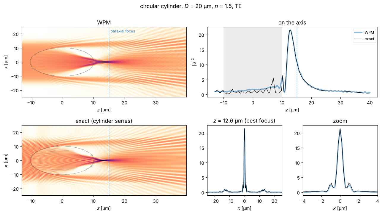
The WPM reproduces the caustic, the position of the best focus (2.6 µm behind the cylinder, well before the paraxial focus because of the spherical aberration) and the transverse profile with its side lobes to about 1 %. The exact solution additionally shows interference fringes: in front of the cylinder between the incident and the reflected light, and inside it with the light reflected at the back surface. The WPM is a one-way method and has neither.

Now the ball lens, with full 2D fields. The 3D field would need a lot of memory, so we step with wpm_propagate() and keep only the \(xz\) cut through the centre. At \(D = 20\lambda\) the exact solution hits a whispering gallery resonance (order \(l = 67\)): a mode that circulates just inside the surface. Its strength changes completely within a few parts per thousand of the wavelength, and it makes the hot spots inside the ball much brighter. A real source has some bandwidth, so we average the exact intensity over a 1.2 % wavelength band, about one spacing of the resonances (11 wavelengths, about half a minute). The WPM, without reflections, has no resonances and hardly depends on the wavelength.

# --- ball lens: WPM with 2D fields ---------------------------------------------------
Ls, Ns, dzs = 80.0, 320, 0.1
xs = grid1d(-Ls/2, Ls/2, Ns)
Xs, Ys = np.meshgrid(xs, xs)
KXs, KYs = np.meshgrid(*(2*np.pi*np.fft.fftfreq(Ns, xs[1] - xs[0]),)*2)
n_sph = lambda X, Y, z: np.where(X**2 + Y**2 + z**2 < a_ball**2, n_ball, 1.0)

def wpm_ball(w, z_end):
    """WPM through the ball for the flat top of radius w; returns z, the xz cut and the field at z_end."""
    u = np.fft.fftshift(back_propagate(np.fft.ifftshift(flat_top(np.hypot(Xs, Ys), w)), KXs, KYs, z0b))
    z_vals = np.arange(z0b, z_end + 1e-9, dzs)
    cut = np.empty((len(z_vals), Ns), dtype=complex)
    cut[0] = u[Ns//2]
    for k in range(1, len(z_vals)):
        u = wpm_propagate(n_sph, u, xs, xs, z_vals[k - 1], dzs, wl)
        cut[k] = u[Ns//2]
    return z_vals, cut

def exact_ball(rho, z, w, wavelengths):
    """Exact (scalar) solution for the same flat top: mean intensity over the wavelengths."""
    r_q = np.linspace(0, 3*w, 3001)
    k_rho = (np.arange(500) + 0.5)*0.005          # radial wavenumbers [1/µm]
    A = (flat_top(r_q, w)*r_q) @ j0(np.outer(r_q, k_rho))*(r_q[1] - r_q[0])   # Hankel transform
    return np.mean([np.abs(sphere_field(rho, z, a_ball, n_ball, wl_j, k_rho=k_rho, amplitudes=A*k_rho*0.005))**2
                    for wl_j in wavelengths], axis=0)

t0 = time.time()
z_s, cut_s = wpm_ball(15.0, 30.0)
print(f"ball lens: {len(z_s) - 1} WPM steps on {Ns}x{Ns}: {time.time() - t0:.1f} s")

band = wl*(1 + np.linspace(-0.006, 0.006, 11))     # 1.2 % wavelength band
z_es, x_es = z_s[::3], xs[np.abs(xs) <= 20]
t0 = time.time()
I_ball_exact = exact_ball(x_es[None, :], z_es[:, None], 15.0, band)
print(f"ball lens: exact solution, {len(band)} wavelengths: {time.time() - t0:.1f} s")

ball lens: 430 WPM steps on 320x320: 6.6 s

ball lens: exact solution, 11 wavelengths: 35.8 s

fig = plt.figure(figsize=(13, 7.2))
gs = fig.add_gridspec(2, 3, width_ratios=[2.2, 1, 1])
ax_w, ax_e = fig.add_subplot(gs[0, 0]), fig.add_subplot(gs[1, 0])
n_map_s = np.array([n_sph(x_es, 0, z) for z in z_es])
sel = np.abs(xs) <= 20
plot_xz(ax_w, cut_s[::3][:, sel], x_es, z_es, n_map=n_map_s, title="WPM, $y$ = 0", gamma=0.4)
plot_xz(ax_e, np.sqrt(I_ball_exact), x_es, z_es, n_map=n_map_s, title="exact (sphere series), $y$ = 0", gamma=0.4)
for ax in (ax_w, ax_e):
    ax.axvline(efl, color="C0", ls="--", lw=1)

ax_ax = fig.add_subplot(gs[0, 1:])
ax_ax.plot(z_s, np.abs(cut_s[:, Ns//2])**2, lw=3, alpha=0.5, label="WPM")
ax_ax.plot(z_es, I_ball_exact[:, len(x_es)//2], "k", lw=0.9, label="exact")
ax_ax.axvspan(-a_ball, a_ball, color="0.92", zorder=-1)
ax_ax.axvline(efl, color="C0", ls="--", lw=1)
ax_ax.set_xlabel("$z$ [µm]"); ax_ax.set_ylabel("$|u|^2$"); ax_ax.set_title("on the axis")
ax_ax.legend(fontsize=9)

k_f = np.argmax(np.where(z_es > a_ball, I_ball_exact[:, len(x_es)//2], 0))
k_fw = np.argmin(np.abs(z_s - z_es[k_f]))
for ax, xl in ((fig.add_subplot(gs[1, 1]), 20), (fig.add_subplot(gs[1, 2]), 3)):
    ax.plot(xs, np.abs(cut_s[k_fw])**2, lw=3, alpha=0.5, label="WPM")
    ax.plot(x_es, I_ball_exact[k_f], "k", lw=0.9, label="exact")
    ax.set_xlim(-xl, xl); ax.set_xlabel("$x$ [µm]")
    ax.set_title(f"$z$ = {z_es[k_f]:.1f} µm (best focus)" if xl > 10 else "zoom")
fig.suptitle(f"ball lens, $D$ = {2*a_ball:.0f} µm, $n$ = {n_ball}", y=1.0)
fig.tight_layout()
I_w = np.abs(cut_s[k_fw, Ns//2])**2
print(f"best focus at z = {z_es[k_f]:.1f} µm (WPM: {z_s[np.argmax(np.where(z_s > a_ball, np.abs(cut_s[:, Ns//2]), 0))]:.1f} µm); "
      f"peak intensity WPM/exact = {I_w/I_ball_exact[k_f, len(x_es)//2]:.3f}")

best focus at z = 12.2 µm (WPM: 12.2 µm); peak intensity WPM/exact = 0.861

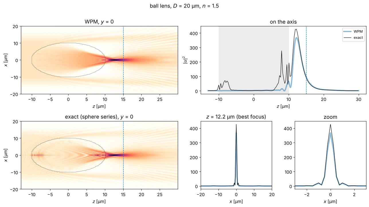
The focus lies at the same place (2.2 µm behind the ball) and has the same width, but the WPM peak is about 14 % too low. On the axis inside the ball, the exact solution shows two hot spots that the WPM misses entirely: the back surface acts as a concave mirror for the 4 % that it reflects and focuses them at \(z \approx 8\) µm, and a second hot spot near the front surface also stems from internally reflected light. On the axis of a sphere, all of a ring’s light adds up in phase, so even weak reflected light becomes bright there. These hot spots inside large spheres are well known from Mie theory (Benincasa et al.). In the cylinder, the same light only forms the weak fringes.

Where does the deficit at the focus come from? The ball lens collects its light from an annulus, and on the axis the weight of each ring grows with its radius: the rim, where the surface is steep, dominates. Narrowing the flat top shows how the error depends on the illuminated aperture (a few seconds per beam):

widths = np.array([5.0, 6.5, 8.0, 9.5, 11.0, 13.0, 15.0])
ratio, z_peaks = [], []
t0 = time.time()
for w in widths:
    z_w, cut_w = wpm_ball(w, 20.0)
    I_w = np.abs(cut_w[:, Ns//2])**2
    behind = z_w > a_ball
    I_e = exact_ball(0*z_w[behind], z_w[behind], w, band)
    ratio.append(I_w[behind].max()/I_e.max())
    z_peaks.append((z_w[behind][np.argmax(I_w[behind])], z_w[behind][np.argmax(I_e)]))
print(f"{len(widths)} beam radii: {time.time() - t0:.1f} s")
ratio, z_peaks = np.array(ratio), np.array(z_peaks)
t_normal = (2/(1 + n_ball))*(2*n_ball/(1 + n_ball))   # amplitude transmission of both surfaces, normal incidence

fig, ax = plt.subplots(figsize=(7, 3.6))
ax.plot(widths/a_ball, ratio, "o-")
ax.axhline(1/t_normal**2, color="gray", ls="--", lw=1)
ax.text(widths[-1]/a_ball, 1/t_normal**2 - 0.012, "no reflection losses (normal incidence): $1/(t_1 t_2)^2$",
        color="gray", fontsize=9, ha="right", va="top")
ax.set_ylim(0.82, 1.12)
ax.axhline(1, color="k", lw=0.6)
ax.set_xlabel("radius of the flat top / radius of the ball, $w/a$")
ax.set_ylabel("peak intensity WPM / exact")
ax.set_title("ball lens: WPM error vs. illuminated aperture")
fig.tight_layout()
for w, r_i, (zw, ze) in zip(widths, ratio, z_peaks):
    print(f"w/a = {w/a_ball:.2f}: WPM/exact = {r_i:.3f}, focus {zw - a_ball:.1f} µm (WPM) / {ze - a_ball:.1f} µm (exact) behind the ball")

7 beam radii: 41.1 s
w/a = 0.50: WPM/exact = 1.060, focus 1.8 µm (WPM) / 1.8 µm (exact) behind the ball
w/a = 0.65: WPM/exact = 0.996, focus 2.8 µm (WPM) / 2.8 µm (exact) behind the ball
w/a = 0.80: WPM/exact = 0.944, focus 2.8 µm (WPM) / 2.7 µm (exact) behind the ball
w/a = 0.95: WPM/exact = 0.899, focus 2.5 µm (WPM) / 2.4 µm (exact) behind the ball
w/a = 1.10: WPM/exact = 0.875, focus 2.4 µm (WPM) / 2.2 µm (exact) behind the ball
w/a = 1.30: WPM/exact = 0.861, focus 2.3 µm (WPM) / 2.1 µm (exact) behind the ball
w/a = 1.50: WPM/exact = 0.856, focus 2.2 µm (WPM) / 2.1 µm (exact) behind the ball

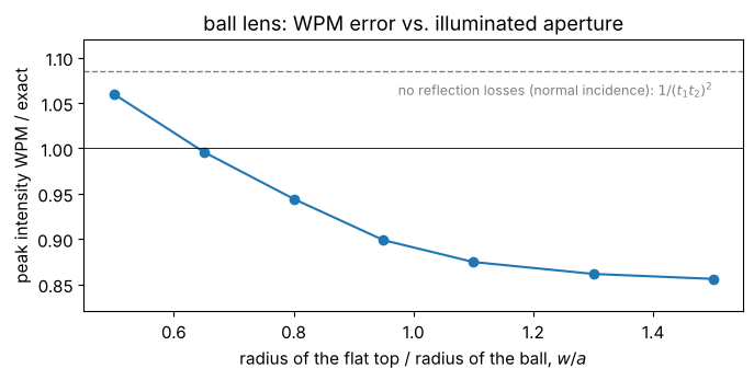
For the central part of the lens (\(w/a \lesssim 0.5\), angles of incidence up to 30°) the WPM is too bright by about the reflection losses it ignores, \(1/(t_1 t_2)^2 = 1.085\). With the rim zone, where the surface is inclined by more than about 50°, the WPM loses light and ends up some 14 % too low; there the local plane wave picture of the WPM is a poor approximation for the strongly tilted interface. In the cylinder the rim has less weight and the two errors happen to cancel. The position and the shape of the focus stay right throughout.

So the WPM gets the geometry of a thick, strongly aberrated lens right, including the caustic and the focus shift, and the intensity to about 10 %, without reflection losses. For more, include the Fresnel losses (e.g. by a ray trace, notebook 19) or use a rigorous method. For small spheres of a few wavelengths (photonic nanojets) or high indices, reflections and resonances matter even more; sphere_field() and cylinder_field() are the reference to check against.

Applications

With the fast "levels" sum, structures made of a few materials cost only a few FFTs per step, so devices that are hundreds of wavelengths long run in seconds. The following sections show some classic applications: integrated optical components, a fibre, a microlens array and a diffraction grating. Wherever possible, the WPM is compared with an independent result.

Two helpers first:

• slab_modes() finds the guided modes of a \(y\)-invariant index profile \(n(x)\) with finite differences, i.e. the eigenvalues \(\beta^2\) of \(\partial_x^2 + k_0^2 n(x)^2\). They serve as input fields and as reference.

• absorber() adds an absorbing index \(i\kappa\) near the window edges, so that radiated light does not re-enter on the other side. \(\kappa\) increases in a few steps instead of smoothly: this keeps the number of distinct index values (and the cost of "levels") small.

from scipy.linalg import eigh_tridiagonal

def slab_modes(n_x, x, num=1):
    # largest eigenvalues beta**2 of d²/dx² + k0² n(x)² (second order finite differences)
    dx = x[1] - x[0]
    diag = -2/dx**2 + (k0*n_x)**2
    off = np.ones(len(x) - 1)/dx**2
    beta2, modes = eigh_tridiagonal(diag, off, select="i", select_range=(len(x) - num, len(x) - 1))
    modes = modes[:, ::-1].T
    return np.sqrt(beta2[::-1]), modes/np.sqrt(np.sum(np.abs(modes)**2, axis=1, keepdims=True))

def absorber(X, L, width=8.0, kappa=0.02, steps=4):
    # i*kappa in `steps` steps within `width` from the window edges +-L/2
    depth = np.clip((np.abs(X) - (L/2 - width))/width, 0, 1)
    return 1j*kappa*np.ceil(depth*steps)/steps

def power_in_mode(u, mode):
    # fraction of the power of the (normalized) mode that u carries, |<mode|u>|²
    return np.abs(np.vdot(mode, u))**2

n_core, n_clad = 1.50, 1.46   # e.g. a polymer or doped glass waveguide

6. Directional coupler

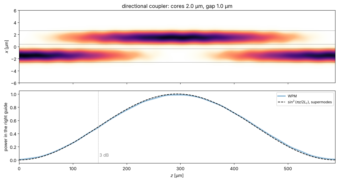
Two parallel waveguides close to each other exchange power: the evanescent tail of the mode in one guide excites the other one. In terms of the supermodes of the pair, light launched into one guide is the sum of the even and the odd supermode, which travel with \(\beta_e\) and \(\beta_o\). Their beating moves the power completely into the other guide after the coupling length

\[L_c = \frac{\pi}{\beta_e - \beta_o}, \qquad P_\mathrm{right}(z) = \sin^2\!\left(\frac{\pi z}{2 L_c}\right).\]

Couplers like this are the basic building block of integrated optics: a coupler of length \(L_c/2\) is a 3 dB splitter (half the power in each output), and it is the beam splitter of integrated Mach-Zehnder interferometers and modulators. Here \(\beta_e\), \(\beta_o\) come from slab_modes() and are compared with the power transfer computed by the WPM.

L5, N5 = 64.0, 512
x5 = grid1d(-L5/2, L5/2, N5)
w_wg, gap = 2.0, 1.0
c = (w_wg + gap)/2   # waveguide centres at +-c
n_pair = lambda X: np.where((np.abs(X - c) <= w_wg/2) | (np.abs(X + c) <= w_wg/2), n_core, n_clad)

(beta_e, beta_o), _ = slab_modes(n_pair(x5), x5, num=2)
L_c = np.pi/(beta_e - beta_o)
_, (mode_left,) = slab_modes(np.where(np.abs(x5 + c) <= w_wg/2, n_core, n_clad), x5)

z_vals = np.arange(0, 2*L_c, 0.5)
t0 = time.time()
U_dc = run_wpm(lambda X, z: n_pair(X) + absorber(X, L5), mode_left, x5, z_vals)
print(f"coupling length from the supermodes: L_c = {L_c:.1f} µm; {len(z_vals) - 1} WPM steps: {time.time() - t0:.1f} s")

I = np.abs(U_dc)**2
P_right = I[:, x5 > 0].sum(axis=1)/I.sum(axis=1)
print(f"WPM: complete transfer at z = {z_vals[np.argmax(P_right)]:.1f} µm, "
      f"3 dB point (50 %) at z = {z_vals[np.argmax(P_right >= 0.5)]:.1f} µm (L_c/2 = {L_c/2:.1f} µm)")

fig, axes = plt.subplots(2, 1, figsize=(12, 6.5), sharex=True)
plot_xz(axes[0], U_dc, x5, z_vals, n_map=np.tile(n_pair(x5), (len(z_vals), 1)),
        title=f"directional coupler: cores {w_wg} µm, gap {gap} µm", xlim=(-6, 6))
axes[0].set_xlabel("")
axes[1].plot(z_vals, P_right, lw=3, alpha=0.5, label="WPM")
axes[1].plot(z_vals, np.sin(np.pi*z_vals/(2*L_c))**2, "k--", label=r"$\sin^2(\pi z/2L_c)$, supermodes")
axes[1].axvline(L_c/2, color="gray", ls=":", lw=1); axes[1].text(L_c/2, 0.05, " 3 dB", color="gray")
axes[1].set_xlabel("$z$ [µm]"); axes[1].set_ylabel("power in the right guide"); axes[1].legend(fontsize=9)
fig.tight_layout()

coupling length from the supermodes: L_c = 294.0 µm; 1176 WPM steps: 1.1 s
WPM: complete transfer at z = 298.5 µm, 3 dB point (50 %) at z = 149.0 µm (L_c/2 = 147.0 µm)

7. Multimode interference (MMI) splitter

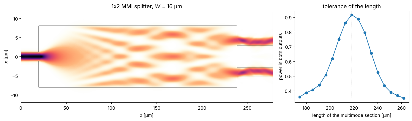
A wide multimode section is fed by a single-mode waveguide. The input excites many modes of the wide section, and since their propagation constants are nearly quadratic in the mode number, \(\beta_0 - \beta_\nu \approx \nu(\nu + 2)\pi/(3L_\pi)\) with the beat length \(L_\pi = \pi/(\beta_0 - \beta_1)\), they rephase periodically: the input field is reproduced as single and multiple self-images. For a centred input, only the symmetric modes are excited and the first two-fold image lies at

\[L_\mathrm{MMI} = \frac{3 L_\pi}{8}.\]

Two output waveguides at \(x = \pm W/4\) pick up the images: a compact, robust 50:50 splitter that is used in most photonic integrated circuits. Scanning the length shows the tolerance of the design.

w_in, W_mmi = 2.0, 16.0
(b0, b1), _ = slab_modes(np.where(np.abs(x5) <= W_mmi/2, n_core, n_clad), x5, num=2)
L_pi = np.pi/(b0 - b1)
L_mmi = 3*L_pi/8
_, (mode_in,) = slab_modes(np.where(np.abs(x5) <= w_in/2, n_core, n_clad), x5)
_, (mode_up,) = slab_modes(np.where(np.abs(x5 - W_mmi/4) <= w_in/2, n_core, n_clad), x5)
_, (mode_down,) = slab_modes(np.where(np.abs(x5 + W_mmi/4) <= w_in/2, n_core, n_clad), x5)
z_in = 20.0   # start of the multimode section

def n_mmi(X, z, length=L_mmi):
    if z < z_in:
        core = np.abs(X) <= w_in/2
    elif z <= z_in + length:
        core = np.abs(X) <= W_mmi/2
    else:
        core = (np.abs(X - W_mmi/4) <= w_in/2) | (np.abs(X + W_mmi/4) <= w_in/2)
    return np.where(core, n_core, n_clad) + absorber(X, L5)

def mmi_outputs(length):
    z = np.arange(0, z_in + length + 40, 0.5)
    U = run_wpm(lambda X, zz: n_mmi(X, zz, length), mode_in, x5, z)
    return z, U, power_in_mode(U[-1], mode_up), power_in_mode(U[-1], mode_down)

z_vals, U_mmi, P_up, P_down = mmi_outputs(L_mmi)
print(f"L_pi = {L_pi:.0f} µm, L_MMI = 3 L_pi/8 = {L_mmi:.1f} µm")
print(f"outputs: {P_up:.3f} / {P_down:.3f}, excess loss {-10*np.log10(P_up + P_down):.2f} dB")

lengths = L_mmi*np.linspace(0.8, 1.2, 17)
P_total = [sum(mmi_outputs(l)[2:]) for l in lengths]

n_map = np.array([n_mmi(x5, z).real for z in z_vals])
fig, axes = plt.subplots(1, 2, figsize=(14, 4.2), gridspec_kw={"width_ratios": [2.2, 1]})
plot_xz(axes[0], U_mmi, x5, z_vals, n_map=n_map, title=f"1x2 MMI splitter, $W$ = {W_mmi:.0f} µm", xlim=(-12, 12))
axes[1].plot(lengths, P_total, "o-")
axes[1].axvline(L_mmi, color="gray", ls=":", lw=1)
axes[1].set_xlabel("length of the multimode section [µm]"); axes[1].set_ylabel("power in both outputs")
axes[1].set_title("tolerance of the length")
fig.tight_layout()

L_pi = 582 µm, L_MMI = 3 L_pi/8 = 218.3 µm
outputs: 0.458 / 0.458, excess loss 0.38 dB

8. Adiabatic taper (spot size converter)

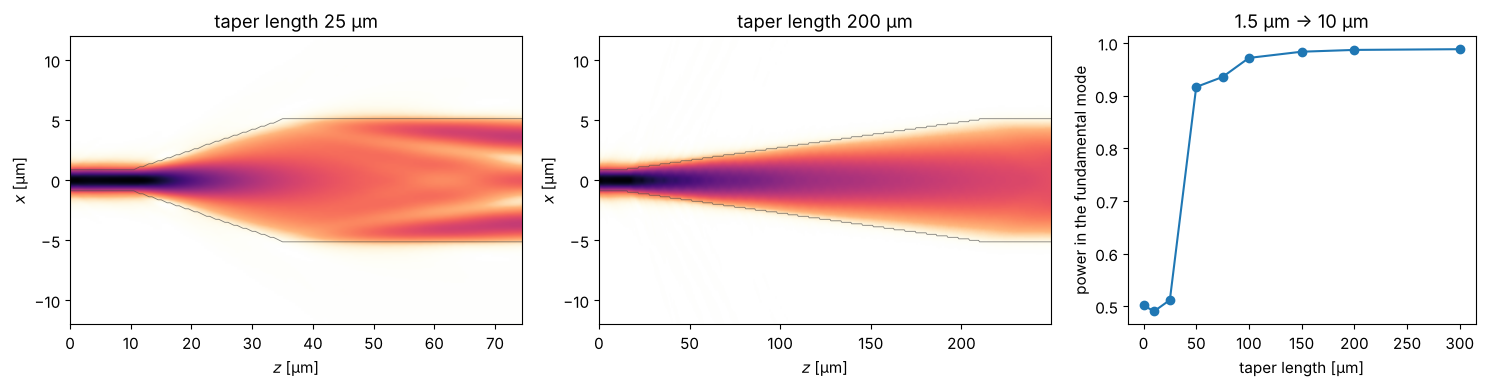
The mode of a narrow waveguide is much smaller than the mode of a fibre or of a wide waveguide. A taper widens the waveguide gradually. If the width changes slowly enough (adiabatically), the light stays in the fundamental mode at every point and arrives in the fundamental mode of the wide guide. An abrupt step instead excites higher order modes and radiation: the coupling efficiency is just the overlap of the two modes. This is how edge couplers bring light from a fibre onto a chip and back.

w_narrow, w_wide, z_start = 1.5, 10.0, 10.0
_, (mode_narrow,) = slab_modes(np.where(np.abs(x5) <= w_narrow/2, n_core, n_clad), x5)
_, (mode_wide,) = slab_modes(np.where(np.abs(x5) <= w_wide/2, n_core, n_clad), x5)

def n_taper(X, z, length):
    s = np.clip((z - z_start)/length, 0, 1) if length > 0 else float(z >= z_start)
    width = w_narrow + (w_wide - w_narrow)*s
    return np.where(np.abs(X) <= width/2, n_core, n_clad) + absorber(X, L5)

def taper(length):
    z = np.arange(0, z_start + length + 40, 0.5)
    U = run_wpm(lambda X, zz: n_taper(X, zz, length), mode_narrow, x5, z)
    return z, U, power_in_mode(U[-1], mode_wide)

taper_lengths = [0, 10, 25, 50, 75, 100, 150, 200, 300]
eta = [taper(l)[2] for l in taper_lengths]
print(f"abrupt step: {eta[0]:.3f} (mode overlap: {power_in_mode(mode_narrow, mode_wide):.3f})")

fig, axes = plt.subplots(1, 3, figsize=(15, 4), gridspec_kw={"width_ratios": [1.3, 1.3, 1]})
for ax, length in zip(axes[:2], (25, 200)):
    z, U, _ = taper(length)
    n_map = np.array([n_taper(x5, zz, length).real for zz in z])
    plot_xz(ax, U, x5, z, n_map=n_map, title=f"taper length {length} µm", xlim=(-12, 12), gamma=0.6)
axes[2].plot(taper_lengths, eta, "o-")
axes[2].set_xlabel("taper length [µm]"); axes[2].set_ylabel("power in the fundamental mode")
axes[2].set_title(f"{w_narrow} µm -> {w_wide:.0f} µm")
fig.tight_layout()

abrupt step: 0.502 (mode overlap: 0.493)

9. Step-index fibre: a full 2D cross-section

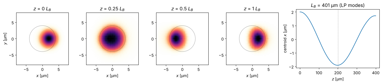
So far all problems were invariant in \(y\). With 2D fields, the WPM propagates through a fibre with a circular core. The guided LP modes of the weakly guiding fibre are known semi-analytically (pyoptics.modes.lp_modes()); the WPM must propagate the LP\(_{01}\) mode unchanged, with the phase velocity given by its effective index \(n_\mathrm{eff}\). A beam launched off-axis excites LP\(_{01}\) and LP\(_{11}\), which beat: the spot swings to the other side of the core after half the beat length \(L_B = \lambda/(n_{\mathrm{eff},01} - n_{\mathrm{eff},11})\). Mode beating like this is the principle of fibre sensors and of the “speckle” of few-mode fibres.

from pyoptics.modes import coupling_efficiency, lp_modes, lp_mode_field
from pyoptics.utils import grid2d

a_core, n1_fib, n2_fib = 4.0, 1.4504, 1.4447
lp01, lp11 = lp_modes(core_radius=a_core, n_core=n1_fib, n_clad=n2_fib, wavelength=wl)
print(f"V = {lp01.V:.2f}: LP01 n_eff = {lp01.n_eff:.6f}, LP11 n_eff = {lp11.n_eff:.6f}")

L8, N8 = 40.0, 128
x8, y8, X8, Y8 = grid2d(-L8/2, L8/2, -L8/2, L8/2, N8, assume_periodicity=True)
n_fibre = lambda X, Y, z: np.where(X**2 + Y**2 <= a_core**2, n1_fib, n2_fib)

# LP01 propagates unchanged; its phase (relative to the cladding) gives n_eff:
u01 = lp_mode_field(lp01, x8, y8, a_core)
z_vals = np.arange(0, 201, 2.0)
U01 = wpm_propagate_z(n_fibre, u01, x8, y8, z_vals, wl)
c01 = np.array([np.vdot(u01, u) for u in U01])
slope = np.polyfit(z_vals, np.unwrap(np.angle(c01*np.exp(-1j*k0*n2_fib*z_vals))), 1)[0]
print(f"WPM: n_eff = {n2_fib + slope/k0:.6f}, power in LP01 after {z_vals[-1]:.0f} µm: "
      f"{coupling_efficiency(U01[-1], u01, x8, y8):.4f}")

# off-axis launch: LP01 and LP11 beat
L_B = wl/(lp01.n_eff - lp11.n_eff)
z_vals = np.arange(0, L_B + 1, 2.0)
t0 = time.time()
U_off = wpm_propagate_z(n_fibre, np.exp(-((X8 - 2.0)**2 + Y8**2)/3.0**2), x8, y8, z_vals, wl)
print(f"{len(z_vals) - 1} WPM steps on {N8}x{N8}: {time.time() - t0:.1f} s")
I = np.abs(U_off)**2
x_centroid = np.sum(I*X8, axis=(1, 2))/np.sum(I, axis=(1, 2))

fig, axes = plt.subplots(1, 5, figsize=(15, 3.4), gridspec_kw={"width_ratios": [1, 1, 1, 1, 1.6]})
for ax, frac in zip(axes, (0, 0.25, 0.5, 1.0)):
    k = np.argmin(np.abs(z_vals - frac*L_B))
    ax.imshow(I[k], extent=(x8[0], x8[-1], y8[0], y8[-1]), cmap=light)
    ax.add_patch(plt.Circle((0, 0), a_core, fill=False, color="0.3", lw=0.6, ls="--"))
    ax.set_xlim(-8, 8); ax.set_ylim(-8, 8); ax.set_title(f"$z$ = {frac:g} $L_B$")
    ax.set_xlabel("$x$ [µm]")
axes[0].set_ylabel("$y$ [µm]")
axes[4].plot(z_vals, x_centroid)
axes[4].axvline(L_B/2, color="gray", ls=":", lw=1)
axes[4].set_xlabel("$z$ [µm]"); axes[4].set_ylabel("centroid $x$ [µm]")
axes[4].set_title(f"$L_B$ = {L_B:.0f} µm (LP modes)")
fig.tight_layout()

V = 3.23: LP01 n_eff = 1.448614, LP11 n_eff = 1.446119

WPM: n_eff = 1.448600, power in LP01 after 200 µm: 0.9977

200 WPM steps on 128x128: 1.0 s

10. Microlens array and Talbot self-imaging

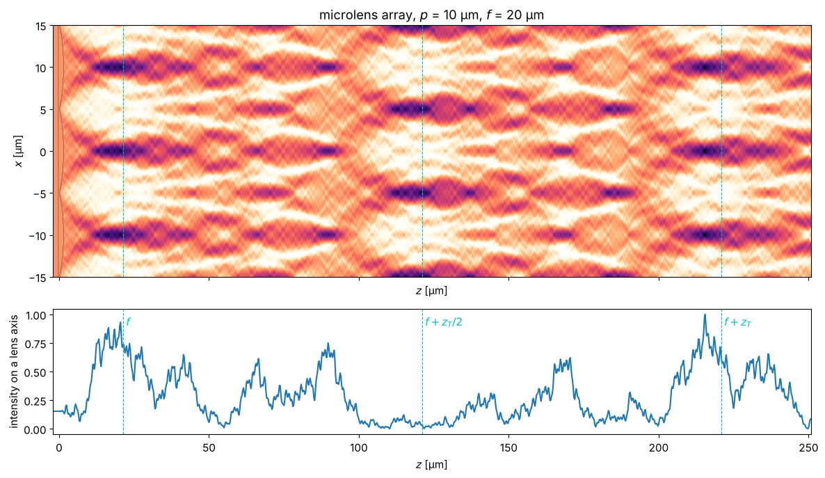
An array of plano-convex cylindrical microlenses (pitch \(p\), radius of curvature \(R\)) focuses a plane wave into a row of foci at \(f = R/(n - 1)\) behind the curved surfaces. Microlens arrays are used in beam homogenizers, Shack-Hartmann sensors (notebook 25) and in front of image sensors. The periodic window of the WPM is convenient here: it represents an infinite array.

Any periodic field reproduces itself after the Talbot length \(z_T \approx 2p^2/\lambda\): the foci reappear near \(f + z_T\) and, shifted by half a pitch, near \(f + z_T/2\); in between lie fractional images. (Strictly, the self-images are exact only in the paraxial limit; the formula \(z_T = \lambda/(1 - \sqrt{1 - \lambda^2/p^2})\) used below is exact for the first harmonic.) The “Talbot carpet” causes crosstalk behind lenslet arrays, and Talbot illuminators use it on purpose. The foci are long: the depth of focus \(\approx \lambda/\mathrm{NA}^2\) of these small lenses is comparable to \(f\).

pitch, R_ml, n_ml, n_lenslets = 10.0, 10.0, 1.5, 6
f_ml = R_ml/(n_ml - 1)
L9 = n_lenslets*pitch
x9 = grid1d(-L9/2, L9/2, 768)
t_ml = R_ml - np.sqrt(R_ml**2 - (pitch/2)**2)   # sag at the lenslet edges

def n_mla(X, z):
    x_local = (X + pitch/2) % pitch - pitch/2   # coordinate within each lenslet
    sag = R_ml - np.sqrt(R_ml**2 - x_local**2)
    return np.where((z >= 0) & (z <= t_ml - sag), n_ml, 1.0)

z_T = wl/(1 - np.sqrt(1 - (wl/pitch)**2))
z_vals = np.arange(-2, t_ml + f_ml + 1.15*z_T, 0.25)
t0 = time.time()
U_mla = run_wpm(n_mla, np.ones_like(x9), x9, z_vals)
print(f"{len(z_vals) - 1} WPM steps: {time.time() - t0:.1f} s; f = {f_ml:.0f} µm, z_T = {z_T:.1f} µm (2p²/λ = {2*pitch**2/wl:.0f} µm)")
I_axis = np.abs(U_mla[:, np.argmin(np.abs(x9))])**2
near = z_vals < t_ml + 1.5*f_ml
print(f"first focus at z = {z_vals[near][np.argmax(I_axis[near])]:.1f} µm (vertex + f = {t_ml + f_ml:.1f} µm)")

n_map = np.array([n_mla(x9, z) for z in z_vals])
fig, axes = plt.subplots(2, 1, figsize=(12, 7), sharex=True, gridspec_kw={"height_ratios": [2, 1]})
plot_xz(axes[0], U_mla, x9, z_vals, n_map=n_map, title=f"microlens array, $p$ = {pitch:.0f} µm, $f$ = {f_ml:.0f} µm",
        xlim=(-1.5*pitch, 1.5*pitch), gamma=0.8)
axes[1].plot(z_vals, I_axis/I_axis.max())
for ax in axes:
    for z_mark, label in ((t_ml + f_ml, "$f$"), (t_ml + f_ml + z_T/2, "$f + z_T/2$"), (t_ml + f_ml + z_T, "$f + z_T$")):
        ax.axvline(z_mark, color="c", ls="--", lw=0.8)
        if ax is axes[1]:
            ax.text(z_mark, 0.9, " " + label, color="c")
axes[1].set_xlabel("$z$ [µm]"); axes[1].set_ylabel("intensity on a lens axis")
fig.tight_layout()

1011 WPM steps: 0.3 s; f = 20 µm, z_T = 199.5 µm (2p²/λ = 200 µm)
first focus at z = 20.5 µm (vertex + f = 21.3 µm)

11. Diffraction gratings: beyond the thin element approximation

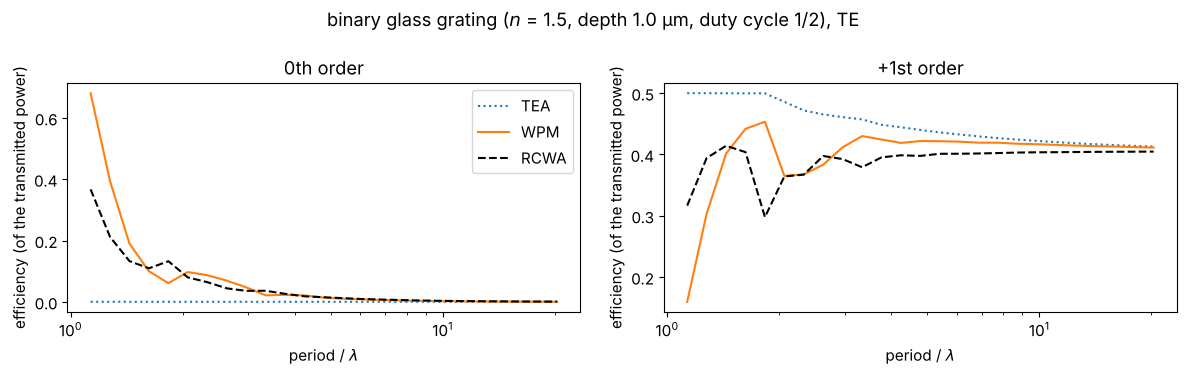
Diffractive optical elements are usually designed with the thin element approximation (TEA): the element multiplies the field by \(e^{i k_0 n(x) d}\). A binary glass grating of depth \(d = \lambda/(2(n - 1))\) and duty cycle 1/2 is then a \(\pi\) phase grating with no zeroth order and \(4/\pi^2 \approx 40.5\,\%\) in each first order. For periods of a few wavelengths, light inside the ridges “sees” the sidewalls and the TEA fails.

The WPM propagates through the grating profile slice by slice and captures most of this. The reference is the rigorous coupled wave analysis (pyoptics.litho.rcwa, TE polarization: \(E\) along the grooves, the scalar case). The efficiencies are normalized to the transmitted power, because the scalar methods ignore reflections. The TEA misses the zeroth order and overestimates the first orders already at periods of \(10\lambda\). The WPM follows RCWA down to periods of about \(3\lambda\) and roughly down to \(2\lambda\); below, the scalar picture breaks down and only RCWA is reliable.

from pyoptics.litho.rcwa import rcwa, Layer

n_gr = 1.5
depth = wl/(2*(n_gr - 1))

def order_efficiencies(field, period, n_out):
    # power flux of the propagating orders, normalized to the transmitted power
    m = np.rint(np.fft.fftfreq(len(field), 1/len(field))).astype(int)
    kz = np.sqrt(complex(1)*((n_out*k0)**2 - (2*np.pi*m/period)**2))
    flux = np.abs(np.fft.fft(field))**2*np.where(np.abs(kz.imag) < 1e-12, kz.real, 0)
    flux = flux/flux.sum()
    return flux[m == 0][0], flux[m == 1][0]

periods = np.geomspace(1.13, 20.3, 25)
eta = {"TEA": [], "WPM": [], "RCWA": []}
for period in periods:
    xg = (np.arange(128) - 64)*period/128
    ridge = np.abs(xg) < period/4
    # plane wave from air through the ridges (z = 0..depth) into the glass substrate:
    u = wpm_propagate_z(lambda X, Y, z: np.where(np.abs(X) < period/4, n_gr, 1.0), np.ones(128, complex),
                        xg, None, np.linspace(0, depth, 41), wl)[-1]
    eta["WPM"].append(order_efficiencies(u, period, n_gr))
    eta["TEA"].append(order_efficiencies(np.exp(1j*k0*np.where(ridge, n_gr, 1.0)*depth), period, n_gr))
    with np.errstate(divide="ignore", invalid="ignore"):
        res = rcwa(period, [Layer(depth, 1.0, [(0.0, period/2, n_gr)])], wl, n_in=1.0, n_out=n_gr, n_orders=40)
        _, T = res.efficiencies((0, 1))   # TE: E_y
    T = T[0]/T[0].sum()
    eta["RCWA"].append((T[res.m == 0][0], T[res.m == 1][0]))

fig, axes = plt.subplots(1, 2, figsize=(12, 3.8), sharex=True)
for name, style in (("TEA", ":"), ("WPM", "-"), ("RCWA", "k--")):
    e = np.array(eta[name])
    axes[0].plot(periods/wl, e[:, 0], style, label=name)
    axes[1].plot(periods/wl, e[:, 1], style, label=name)
for ax, title in zip(axes, ("0th order", "+1st order")):
    ax.set_xscale("log"); ax.set_xlabel(r"period / $\lambda$"); ax.set_title(title)
    ax.set_ylabel("efficiency (of the transmitted power)")
axes[0].legend()
fig.suptitle(f"binary glass grating ($n$ = {n_gr}, depth {depth:.1f} µm, duty cycle 1/2), TE")
fig.tight_layout()

12. Limits

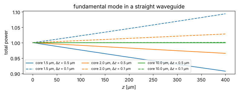
The WPM is a scalar method. It neglects reflections and polarization, and at sharp index steps it does not conserve power exactly: the local plane wave sum is not a unitary operation. In waveguides, where the light meets the core boundary over and over, this shows up as a slow drift of the power. The check below propagates the fundamental mode of straight guides: the drift is largest for narrow, strongly confined cores, its size and even its sign depend on the step \(\Delta z\), and it does not vanish for \(\Delta z \to 0\). In the examples above (step 0.5 µm), the losses of the narrow guides are partly this numerical loss, e.g. a part of the excess loss of the MMI. Wide guides and smooth (GRIN) profiles are not affected.

For high index contrast (silicon photonics), sub-wavelength structures or polarization dependent problems, a full-vector method (RCWA, FDTD, vectorial mode solvers) is the right tool. The WPM is excellent for weakly guiding structures, lenses, gradient index media and moderately thick diffractive elements.

fig, ax = plt.subplots(figsize=(8, 3.2))
for width, color in ((1.5, "C0"), (2.0, "C1"), (10.0, "C2")):
    n_x = np.where(np.abs(x5) <= width/2, n_core, n_clad)
    _, (mode,) = slab_modes(n_x, x5)
    for dz, ls in ((0.5, "-"), (0.1, "--")):
        z_vals = np.arange(0, 400 + dz/2, dz)
        U = run_wpm(lambda X, z: n_x, mode, x5, z_vals)
        ax.plot(z_vals, np.sum(np.abs(U)**2, axis=1), ls, color=color,
                label=f"core {width} µm, $\\Delta z$ = {dz} µm")
ax.set_xlabel("$z$ [µm]"); ax.set_ylabel("total power"); ax.legend(fontsize=8, ncol=3, loc="lower left")
ax.set_title("fundamental mode in a straight waveguide")
fig.tight_layout()

References

• K.-H. Brenner and W. Singer, “Light propagation through microlenses: a new simulation method”, Appl. Opt. 32, 4984-4988 (1993).

• S. Schmidt, T. Tiess, S. Schröter, R. Hambach, M. Jäger, H. Bartelt, A. Tünnermann and H. Gross, “Wave-optical modeling beyond the thin-element-approximation”, Opt. Express 24, 30188 (2016).

• M. D. Feit and J. A. Fleck, “Light propagation in graded-index optical fibers”, Appl. Opt. 17, 3990-3998 (1978).

• L. B. Soldano and E. C. M. Pennings, “Optical multi-mode interference devices based on self-imaging: principles and applications”, J. Lightwave Technol. 13, 615-627 (1995).

• A. W. Snyder and J. D. Love, Optical Waveguide Theory, Chapman and Hall (1983).

• H. F. Talbot, “Facts relating to optical science. No. IV”, Phil. Mag. 9, 401 (1836).

• G. Mie, “Beiträge zur Optik trüber Medien, speziell kolloidaler Metallösungen”, Ann. Phys. 330, 377-445 (1908).

• C. F. Bohren and D. R. Huffman, Absorption and Scattering of Light by Small Particles, Wiley (1983), chapters 4 (sphere) and 8 (cylinder).

• J. R. Wait, “Scattering of a plane wave from a circular dielectric cylinder at oblique incidence”, Can. J. Phys. 33, 189-195 (1955).

• P. M. Morse and K. U. Ingard, Theoretical Acoustics, McGraw-Hill (1968) (scattering of scalar waves by a sphere).

• G. Gouesbet and G. Gréhan, Generalized Lorenz-Mie Theories, Springer (2011).

• W. J. Wiscombe, “Improved Mie scattering algorithms”, Appl. Opt. 19, 1505-1509 (1980).

• D. S. Benincasa, P. W. Barber, J.-Z. Zhang, W.-F. Hsieh and R. K. Chang, “Spatial distribution of the internal and near-field intensities of large cylindrical and spherical scatterers”, Appl. Opt. 26, 1348-1356 (1987).

• E. Hecht, Optics, 5th ed., Pearson (2017), chapter 6 (thick lenses).