Imaging, resolution and aberrations

This notebook combines pyoptics.imaging (coherent imaging through a 4f system with numerical aperture NA), pyoptics.bases (Fringe Zernike polynomials for wavefront errors) and pyoptics.propagators (three-dimensional point spread function). Topics: Zernike gallery, point spread function (PSF) with aberrations, Strehl ratio and Maréchal approximation, Zernike fit, coherent and incoherent imaging, the Rayleigh criterion and the focus in 3D. Notebook 16 looks at the basis functions themselves in more depth.

import numpy as np
import matplotlib.pyplot as plt

from pyoptics import imaging
from pyoptics import propagators as prop
from pyoptics.bases import FringeZernikes, fringe_to_n_m
from pyoptics.fft import FT, inv_FT
from pyoptics.masks import circular_mask
from pyoptics.utils import grid2d, freq_grid, wavenumber

plt.rcParams.update({"figure.dpi": 100, "image.origin": "lower", "font.size": 11})

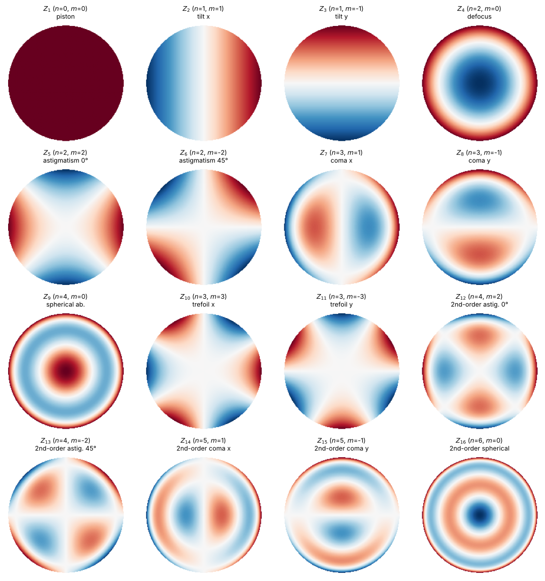
1. Fringe Zernike polynomials

Zernike polynomials \(Z_j(\rho, \varphi)\) are orthogonal on the unit disk and describe the typical aberrations of rotationally symmetric systems. FringeZernikes numbers them in the Fringe order (index starting at 1) and normalizes them to \(|Z_j(\rho = 1)| = 1\).

names = {1: "piston", 2: "tilt x", 3: "tilt y", 4: "defocus", 5: "astigmatism 0°",
         6: "astigmatism 45°", 7: "coma x", 8: "coma y", 9: "spherical ab.", 10: "trefoil x",
         11: "trefoil y", 12: "2nd-order astig. 0°", 13: "2nd-order astig. 45°", 14: "2nd-order coma x",
         15: "2nd-order coma y", 16: "2nd-order spherical"}
xp, yp, _, _ = grid2d(-1.05, 1.05, -1.05, 1.05, 201)
Zb = FringeZernikes(xp, yp)
mask_p = circular_mask(xp, yp, 1.0).astype(bool)

fig, axes = plt.subplots(4, 4, figsize=(11, 11.5))
for ax, j in zip(axes.flat, range(1, 17)):
    Zj = np.where(mask_p, Zb([j], [1.0]), np.nan)
    ax.imshow(Zj, cmap="RdBu_r", vmin=-1, vmax=1, extent=(xp[0], xp[-1], yp[0], yp[-1]))
    n, m = fringe_to_n_m(j)
    ax.set_title(f"$Z_{{{j}}}$ ($n$={n}, $m$={m})\n{names[j]}", fontsize=9)
    ax.axis("off")
fig.tight_layout()

2. Point spread function with aberrations

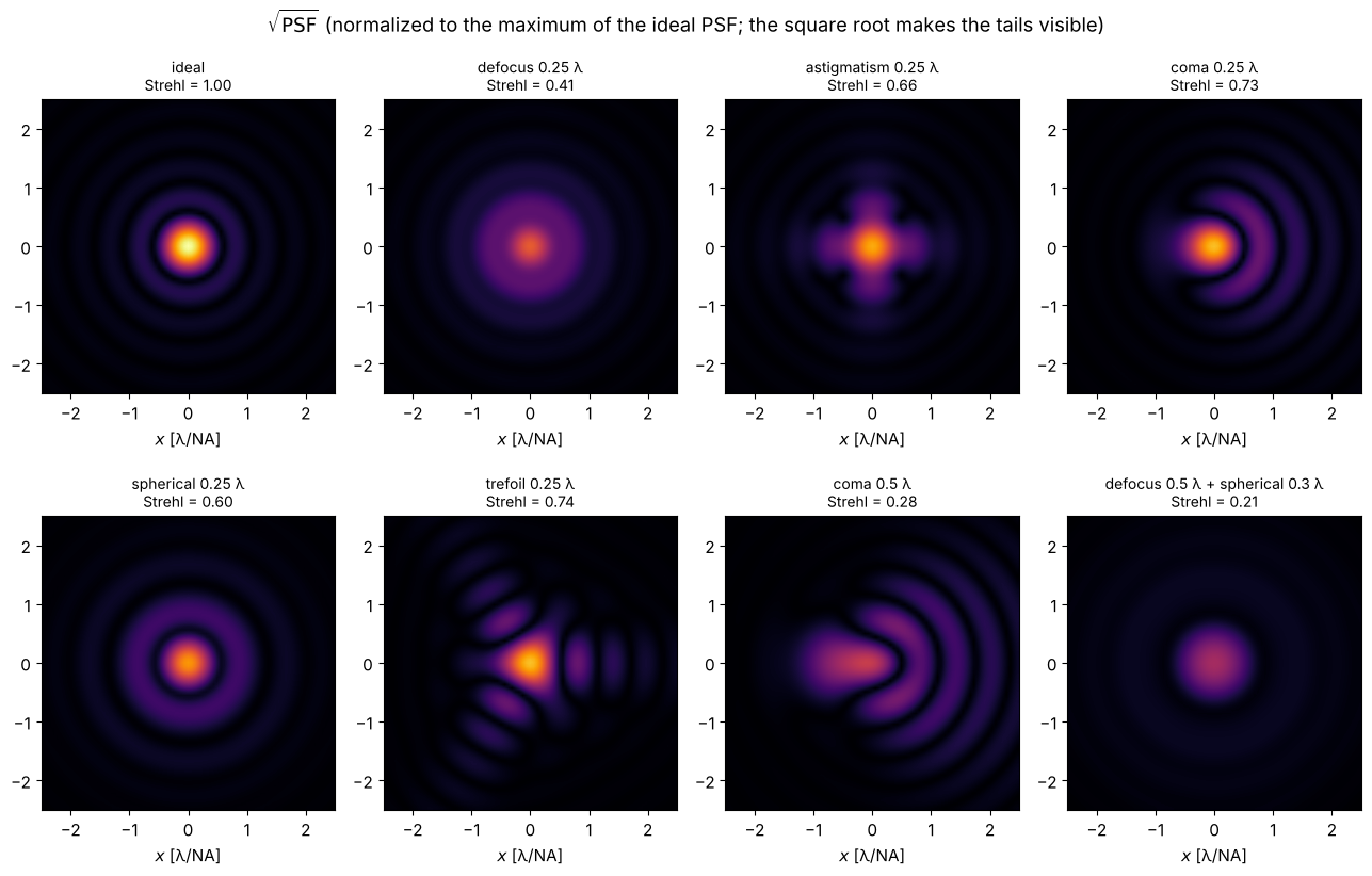
The pupil function is \(P(\rho, \varphi) = \mathrm{circ}(\rho)\, e^{2\pi i W(\rho,\varphi)}\) with the wavefront error \(W = \sum_j c_j Z_j\) in waves. The PSF is the squared modulus of its Fourier transform. Zero padding by a factor of 8 around the pupil samples the PSF finely enough; image coordinates are given in units of \(\lambda/\mathrm{NA}\).

Lp, Np = 16.0, 1024           # pupil coordinates in units of the pupil radius
xq, yq, _, _ = grid2d(-Lp/2, Lp/2, -Lp/2, Lp/2, Np)
Zq = FringeZernikes(xq, yq)
pupil = circular_mask(xq, yq, 1.0).astype(float)
u = np.fft.fftshift(np.fft.fftfreq(Np, xq[1] - xq[0]))  # image coordinate in lambda/NA

def psf(coeffs):
    """coeffs: dict {Fringe index: coefficient in waves}"""
    W = sum(c*Zq([j], [1.0]) for j, c in coeffs.items()) if coeffs else 0.0
    P = pupil*np.exp(2j*np.pi*W)
    return np.abs(FT(P))**2

I_perfect = psf({})
I0 = I_perfect.max()

cases = [({}, "ideal"), ({4: 0.25}, "defocus 0.25 λ"), ({5: 0.25}, "astigmatism 0.25 λ"),
         ({7: 0.25}, "coma 0.25 λ"), ({9: 0.25}, "spherical 0.25 λ"), ({10: 0.25}, "trefoil 0.25 λ"),
         ({7: 0.5}, "coma 0.5 λ"), ({4: 0.5, 9: 0.3}, "defocus 0.5 λ + spherical 0.3 λ")]
c = 2.5
sel = np.abs(u) <= c
fig, axes = plt.subplots(2, 4, figsize=(13, 8.4))
for ax, (coeffs, title) in zip(axes.flat, cases):
    I = psf(coeffs)
    ax.imshow(np.sqrt(I[np.ix_(sel, sel)]/I0), extent=(-c, c, -c, c), cmap="inferno", vmax=1.0, interpolation="bilinear")
    ax.set_title(f"{title}\nStrehl = {I.max()/I0:.2f}", fontsize=10)
    ax.set_xlabel("$x$ [λ/NA]")
fig.suptitle("$\\sqrt{\\mathrm{PSF}}$ (normalized to the maximum of the ideal PSF; the square root makes the tails visible)")
fig.tight_layout()

Strehl ratio and the Maréchal approximation

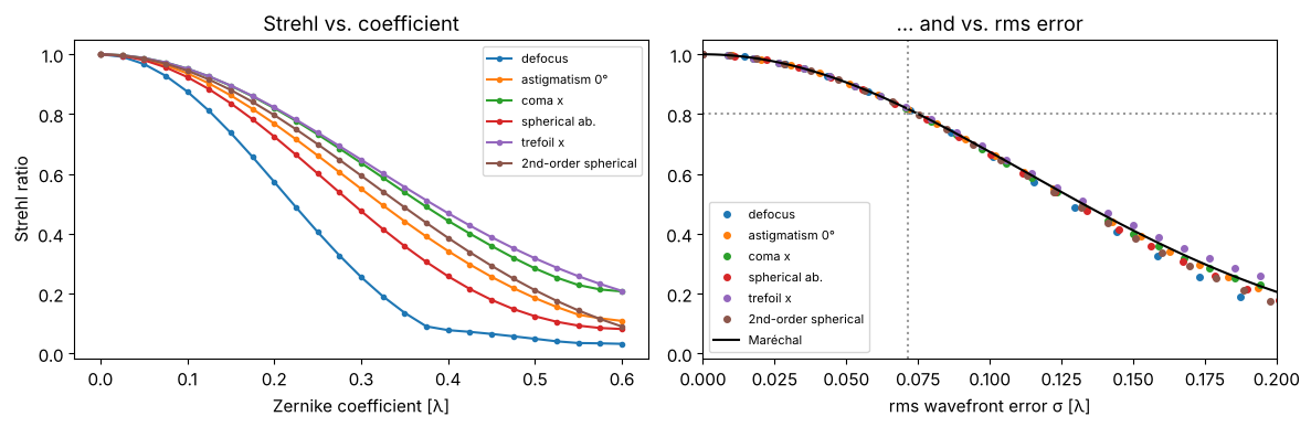
The Strehl ratio is the peak intensity relative to the ideal PSF. For small errors it depends only on the rms wavefront error \(\sigma\), not on the type of aberration:

\[S \approx \exp\big(-(2\pi\sigma)^2\big).\]

A system counts as “diffraction limited” for \(S \geq 0.8\), i.e. \(\sigma \lesssim \lambda/14\) (Maréchal criterion). Note: tilt only shifts the PSF, so we take the maximum of the PSF here rather than its value at the origin.

amps = np.linspace(0, 0.6, 25)
fig, axes = plt.subplots(1, 2, figsize=(12, 4))
for j in (4, 5, 7, 9, 10, 16):
    rms, strehl = [], []
    Zj = Zq([j], [1.0])
    for a in amps:
        rms.append(np.std(a*Zj[pupil > 0]))
        strehl.append(psf({j: a}).max()/I0)
    axes[0].plot(amps, strehl, "o-", ms=3, label=names[j])
    axes[1].plot(rms, strehl, "o", ms=4, label=names[j])
s = np.linspace(0, 0.2, 100)
axes[1].plot(s, np.exp(-(2*np.pi*s)**2), "k-", lw=1.5, label="Maréchal")
axes[1].axhline(0.8, color="0.6", ls=":"); axes[1].axvline(1/14, color="0.6", ls=":")
axes[0].set_xlabel("Zernike coefficient [λ]"); axes[0].set_ylabel("Strehl ratio")
axes[1].set_xlabel("rms wavefront error σ [λ]"); axes[1].set_xlim(0, 0.2)
axes[0].legend(fontsize=8); axes[1].legend(fontsize=8)
axes[0].set_title("Strehl vs. coefficient"); axes[1].set_title("... and vs. rms error")
fig.tight_layout()

3. Zernike fit of a measured wavefront

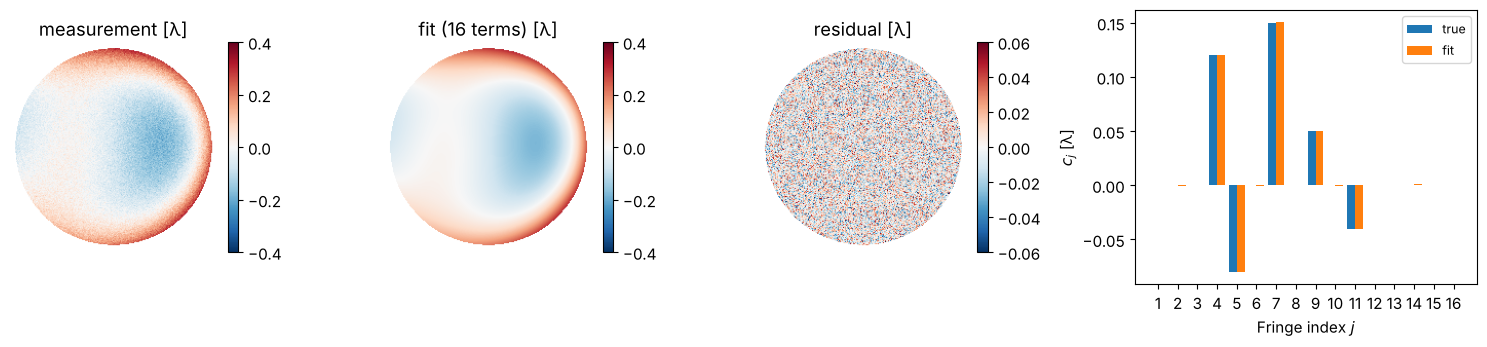
coeffs_from_field() decomposes a wavefront (here: synthetic, with noise) into Zernike polynomials by least squares. The aberrations can be read off directly from the coefficients.

rng = np.random.default_rng(0)
true = {4: 0.12, 5: -0.08, 7: 0.15, 9: 0.05, 11: -0.04}
indices = list(range(1, 17))
W_true = sum(c*Zb([j], [1.0]) for j, c in true.items())
W_meas = W_true + 0.02*rng.standard_normal(W_true.shape)
W_meas_masked = np.where(mask_p, W_meas, 0.0)
coeffs_fit = Zb.coeffs_from_field(W_meas_masked, indices)
W_fit = Zb(indices, coeffs_fit)

fig, axes = plt.subplots(1, 4, figsize=(15, 3.6), gridspec_kw={"width_ratios": [1, 1, 1, 1.5]})
for ax, W, title in zip(axes, (W_meas, W_fit, W_meas - W_fit), ("measurement [λ]", "fit (16 terms) [λ]", "residual [λ]")):
    im = ax.imshow(np.where(mask_p, W, np.nan), cmap="RdBu_r", extent=(xp[0], xp[-1], yp[0], yp[-1]),
                   vmin=-0.4 if title != "residual [λ]" else -0.06, vmax=0.4 if title != "residual [λ]" else 0.06)
    fig.colorbar(im, ax=ax, fraction=0.046); ax.set_title(title); ax.axis("off")
axes[3].bar(np.array(indices) - 0.2, [true.get(j, 0.0) for j in indices], 0.4, label="true")
axes[3].bar(np.array(indices) + 0.2, np.real(coeffs_fit), 0.4, label="fit")
axes[3].set_xticks(indices); axes[3].set_xlabel("Fringe index $j$"); axes[3].set_ylabel("$c_j$ [λ]")
axes[3].legend(fontsize=9)
fig.tight_layout()

4. Coherent and incoherent imaging

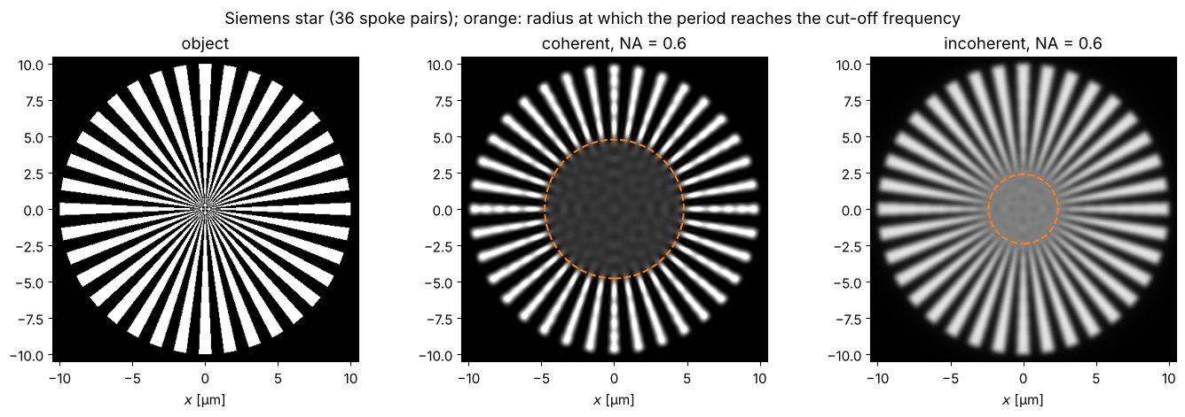
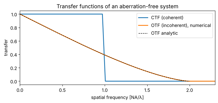
imaging.image() images a (complex) object coherently: the spectrum is cut off at \(|k_\perp| > k\,\mathrm{NA}\). The coherent transfer function (CTF) is thus the pupil itself, with the cut-off frequency \(\mathrm{NA}/\lambda\).

With incoherent illumination (e.g. fluorescence), intensities add. The image is the object intensity convolved with \(|h|^2\), the intensity PSF (from imaging.get_psf()). The optical transfer function (OTF) is the autocorrelation of the pupil and reaches twice as far, up to \(2\mathrm{NA}/\lambda\), but falls off towards high frequencies.

A Siemens star shows both limits directly: the spokes blur towards the centre where their period drops below the resolution limit.

wl, NA = 0.5, 0.6
k = wavenumber(wl)
L, N = 24.0, 512
x, y, X, Y = grid2d(-L/2, L/2, -L/2, L/2, N)
R, PHI = np.hypot(X, Y), np.arctan2(Y, X)
n_spokes = 36
star = ((np.cos(n_spokes*PHI) > 0) & (R < 10)).astype(float)

img_coh = np.abs(imaging.image(star, x, y, NA, k))**2
h = imaging.get_psf(x, y, NA, k)
H_inc = FT(np.abs(h)**2)
img_inc = np.real(inv_FT(FT(star)*H_inc/H_inc[N//2, N//2]))

r_coh = n_spokes*wl/(2*np.pi*NA)      # period 2 pi r / n_spokes = lambda/NA
r_inc = n_spokes*wl/(4*np.pi*NA)      # period = lambda/(2 NA)

fig, axes = plt.subplots(1, 3, figsize=(14, 4.6))
for ax, I, title, r_lim in zip(axes, (star, img_coh, img_inc),
                               ("object", f"coherent, NA = {NA}", f"incoherent, NA = {NA}"),
                               (None, r_coh, r_inc)):
    ax.imshow(I, extent=(x[0], x[-1], y[0], y[-1]), cmap="gray", vmin=0, vmax=1.2 if I is img_coh else 1)
    if r_lim:
        ax.add_patch(plt.Circle((0, 0), r_lim, fill=False, color="C1", lw=1.5, ls="--"))
    ax.set_xlim(-10.5, 10.5); ax.set_ylim(-10.5, 10.5); ax.set_title(title); ax.set_xlabel("$x$ [µm]")
fig.suptitle("Siemens star (36 spoke pairs); orange: radius at which the period reaches the cut-off frequency")
fig.tight_layout()

fx, fy = freq_grid(x, y, wavenumbers=False, normal_order=True)
CTF = (np.hypot(fx, fy) <= NA/wl).astype(float)
OTF = np.abs(H_inc)/np.abs(H_inc).max()
f_axis = fx[N//2]
nu = np.linspace(0, 1, 200)
otf_ana = 2/np.pi*(np.arccos(nu) - nu*np.sqrt(1 - nu**2))
fig, ax = plt.subplots(figsize=(7.5, 3.6))
ax.plot(f_axis*wl/NA, CTF[N//2], lw=2, label="CTF (coherent)")
ax.plot(f_axis*wl/NA, OTF[N//2], lw=2, label="OTF (incoherent), numerical")
ax.plot(2*nu, otf_ana, "k--", lw=1, label="OTF analytic")
ax.set_xlim(0, 2.3); ax.set_xlabel("spatial frequency [NA/λ]"); ax.set_ylabel("transfer")
ax.legend(); ax.set_title("Transfer functions of an aberration-free system")
fig.tight_layout()

5. Two points: the Rayleigh criterion

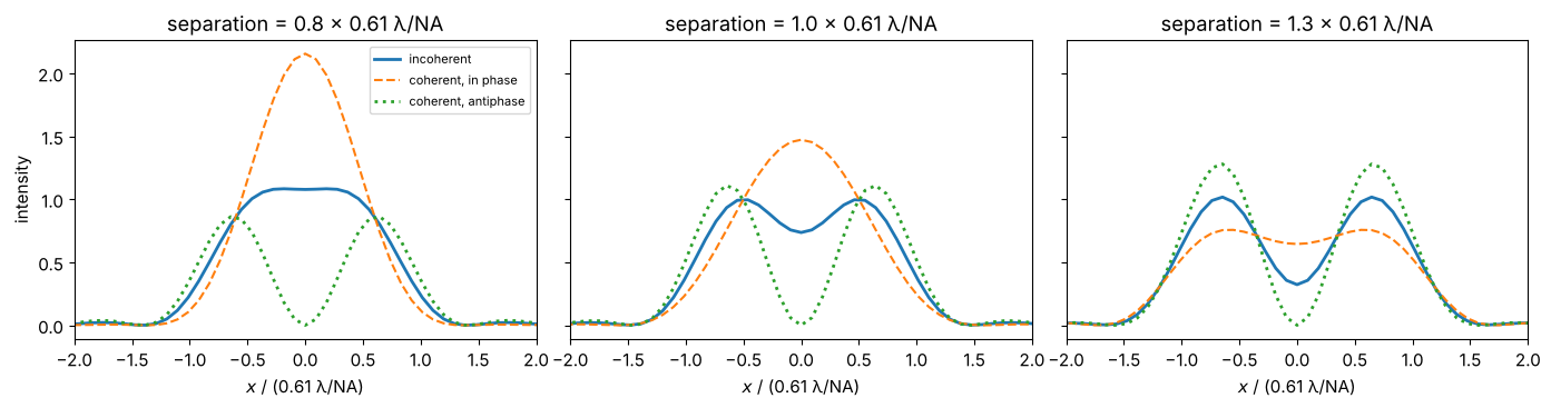
Two incoherent point sources at a distance \(0.61\,\lambda/\mathrm{NA}\) (maximum of one PSF on the first zero of the other) are just resolved, with a dip to about 73 %. With coherent illumination the relative phase decides: points in phase merge, points in antiphase are clearly separated by a dark line (the principle of phase-shift masks in lithography).

d_R = 0.61*wl/NA
KX, KY = freq_grid(x, y, wavenumbers=True, normal_order=True)
fig, axes = plt.subplots(1, 3, figsize=(14, 3.8), sharey=True)
for ax, sep in zip(axes, (0.8*d_R, d_R, 1.3*d_R)):
    shift = lambda f, dx: inv_FT(FT(f)*np.exp(-1j*KX*dx))  # shift by dx via the Fourier shift theorem
    h1, h2 = shift(h, -sep/2), shift(h, +sep/2)
    norm = np.abs(h).max()**2
    ax.plot(x/d_R, (np.abs(h1)**2 + np.abs(h2)**2)[N//2]/norm, lw=2, label="incoherent")
    ax.plot(x/d_R, np.abs(h1 + h2)[N//2]**2/norm, "--", label="coherent, in phase")
    ax.plot(x/d_R, np.abs(h1 - h2)[N//2]**2/norm, ":", lw=2, label="coherent, antiphase")
    ax.set_xlim(-2, 2); ax.set_xlabel("$x$ / (0.61 λ/NA)")
    ax.set_title(f"separation = {sep/d_R:.1f} × 0.61 λ/NA")
axes[0].set_ylabel("intensity"); axes[0].legend(fontsize=8)
fig.tight_layout()

6. The focus in three dimensions

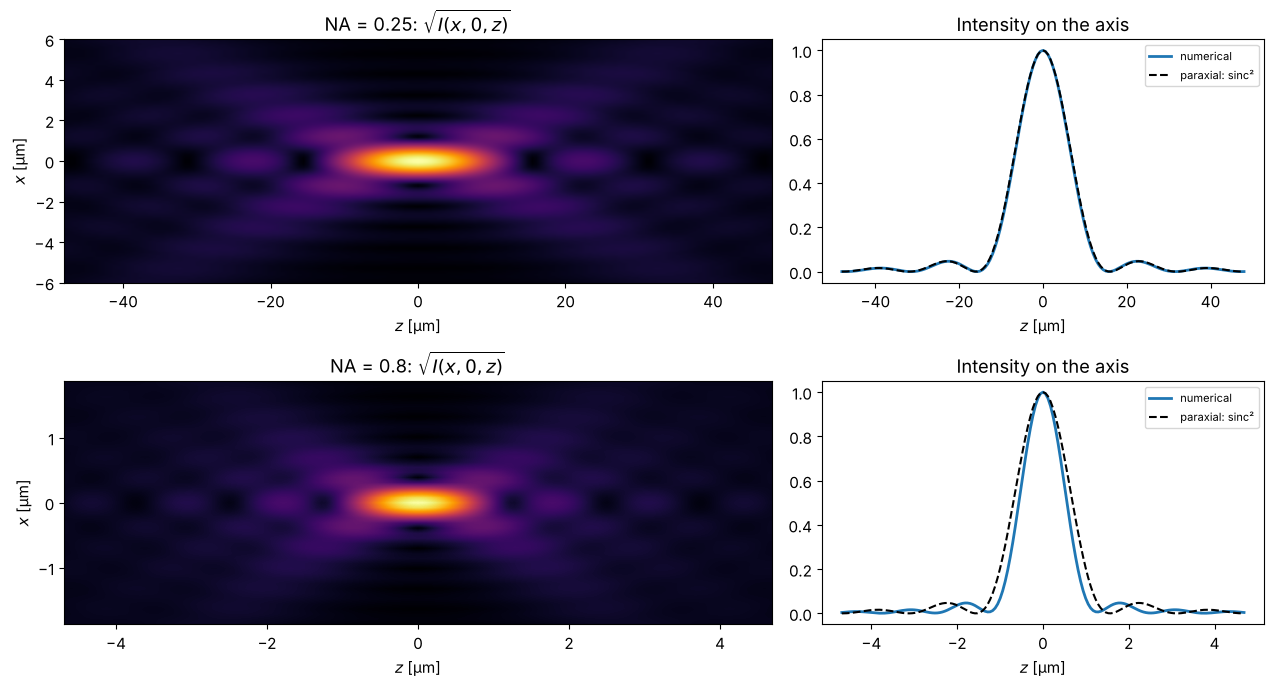
The field in the focal plane is the (amplitude) PSF \(h\). Propagating it forwards and backwards with the exact Rayleigh-Sommerfeld propagator gives the three-dimensional PSF. For small NA, on the axis,

\[I(0, 0, z) = I_0\,\mathrm{sinc}^2\!\left(\frac{\mathrm{NA}^2 z}{2\lambda}\right), \qquad \mathrm{sinc}(x) = \frac{\sin \pi x}{\pi x},\]

with the first zero at \(z = 2\lambda/\mathrm{NA}^2\). At large NA, the focus is shorter than the paraxial formula predicts, because the marginal rays arrive more steeply.

Careful with backward propagation: for \(z < 0\), evanescent components are amplified by \(e^{+|k_z||z|}\). Even rounding errors of \(10^{-16}\) in this frequency range then grow without bound. Time reversal helps: \(U(-z) = \overline{\mathcal{P}_z\big[\overline{U}\big]}\). For propagating waves this is exactly the backward propagation, while evanescent waves are damped instead of amplified.

L3, N3 = 40.0, 512  # window large enough for the defocused cone of light
x3, y3, _, _ = grid2d(-L3/2, L3/2, -L3/2, L3/2, N3)
fig, axes = plt.subplots(2, 2, figsize=(13, 7), gridspec_kw={"width_ratios": [1.6, 1]})
for row, NA3 in enumerate((0.25, 0.8)):
    h3 = imaging.get_psf(x3, y3, NA3, k)
    z_max = 3*2*wl/NA3**2
    z3 = np.linspace(-z_max, z_max, 161)
    def propagate(U, z):
        if z >= 0:
            return prop.rayleigh_sommerfeld_I_TF(U, x3, y3, z, wl)[0]
        return np.conj(prop.rayleigh_sommerfeld_I_TF(np.conj(U), x3, y3, -z, wl)[0])  # time reversal
    stack = np.array([propagate(h3, z)[N3//2] for z in z3])
    I3 = np.abs(stack)**2
    I3 /= I3.max()
    axes[row, 0].imshow(I3.T**0.5, extent=(z3[0], z3[-1], x3[0], x3[-1]), aspect="auto", cmap="inferno",
                        interpolation="bilinear")
    axes[row, 0].set_ylim(-3*wl/NA3, 3*wl/NA3)
    axes[row, 0].set_xlabel("$z$ [µm]"); axes[row, 0].set_ylabel("$x$ [µm]")
    axes[row, 0].set_title(f"NA = {NA3}: $\\sqrt{{I(x, 0, z)}}$")
    axes[row, 1].plot(z3, I3[:, N3//2], lw=2, label="numerical")
    axes[row, 1].plot(z3, np.sinc(NA3**2*z3/(2*wl))**2, "k--", label="paraxial: sinc²")
    axes[row, 1].set_xlabel("$z$ [µm]"); axes[row, 1].set_title("Intensity on the axis"); axes[row, 1].legend(fontsize=8)
fig.tight_layout()

References

• J. W. Goodman, Introduction to Fourier Optics, 4th ed., W. H. Freeman (2017).

• M. Born and E. Wolf, Principles of Optics, 7th ed., Cambridge University Press (1999).

• V. N. Mahajan, Optical Imaging and Aberrations, Part II: Wave Diffraction Optics, 2nd ed., SPIE Press (2011).

• R. J. Noll, “Zernike polynomials and atmospheric turbulence”, J. Opt. Soc. Am. 66, 207-211 (1976).

• J. C. Wyant and K. Creath, “Basic wavefront aberration theory for optical metrology”, in R. R. Shannon and J. C. Wyant (eds.), Applied Optics and Optical Engineering, Vol. XI, Academic Press (1992).

• Lord Rayleigh, “Investigations in optics, with special reference to the spectroscope”, Phil. Mag. 8, 261-274 (1879).